Aug 23, 2012 - For random graphs distributed according to a stochastic block model, we consider the inferential task of partioning vertices into blocks using ...
Consistent adjacency-spectral partitioning for the
arXiv:1205.0309v2 [stat.ME] 21 Aug 2012
stochastic block model when the model parameters are unknown Donniell E. Fishkind, Daniel L. Sussman, Minh Tang, Joshua T. Vogelstein and Carey E. Priebe Department of Applied Mathematics and Statistics, Johns Hopkins University August 23, 2012
Abstract For random graphs distributed according to a stochastic block model, we consider the inferential task of partioning vertices into blocks using spectral techniques. Spectral partioning using the normalized Laplacian and the adjacency matrix have both been shown to be consistent as the number of vertices tend to infinity. Importantly, both procedures require that the number of blocks and the rank of the communication probability matrix are known, even as the rest of the parameters may be unknown. In this article, we prove that the (suitably modified) adjacency-spectral partitioning procedure, requiring only an upper bound on the rank of the communication probability matrix, is consistent. Indeed, this result demonstrates a robustness to model misspecification; an overestimate of the rank may impose a moderate performance penalty, but the procedure is still consistent. Furthermore, we extend this procedure to the setting where adjacencies may have multiple modalities and we allow for either directed or undirected graphs.
1
1
Background and overview
Our setting is the stochastic block model [12, 25]—a random graph model in which a set of n vertices is randomly partitioned into K blocks and then, conditioned on the partition, existence of edges between all pairs of vertices are independent Bernoulli trials with parameters determined by the block membership of the pair. (The model details are specified in Section 2.1.) The realized partition of the vertices is not observed, nor are the Bernoulli trial parameters known. However, the realized vertex adjacencies (edges) are observed, and the main inferential task is to estimate the partition of the vertices, using the realized adjacencies as a guide. Such an estimate will be called consistent if and when, in considering a sequence of realizations for n = 1, 2, 3, . . . with common model parameters, it happens almost surely that the fraction of misassigned vertices converges to zero as n → ∞.
Rohe et al. [20] proved the consistency of a block estimator that is based on spectral
partitioning applied to the normalized Laplacian, and Sussman et al. [24] extended this to prove the consistency of a block estimator that is based on spectral partitioning applied to the adjacency matrix. Importantly, both of these procedures assume that K and the rank of M are known (where M ∈ [0, 1]K×K is the matrix consisting of the Bernoulli parameters for
all pairs of blocks), even as the rest of the parameters may be unknown. In this article, we prove that the (suitably modified) adjacency-spectral partitioning procedure, requiring only
an upper bound for rankM , gives consistent block estimation. We demonstrate a robustness to mis-specification of rankM ; in particular, if a practitioner overestimates the rank of M in carrying out adjacency spectral partitioning to estimate the blocks, then the consistency of the procedure is not lost. Indeed, this is a model selection result, and we provide estimators for K and prove their consistency. Our analysis and results are valid for both directed and undirected graphs. We also allow for more than one modality of adjacency. For instance, the stochastic block model can model a social network in which the vertices are people, and the blocks are different communities within the network such that probabilities of communication between individual people are community dependent, and there is available information about several different modes of communication between the people; e.g. who phoned whom on cell phones, who phoned whom on land lines, who sent email to whom, who sent snail mail to whom, with a separate adjacency matrix for each modality of communication. Indeed, if there are
2
different matrices M for each mode of communication, even if there is dependence in the communications between two people across different modalities, our analysis and results will hold—provided that every pair of blocks is “probabilistically discernable” within at least one mode of communication. (This will be made more precise in Section 2.1.) Latent space models (e.g. Hoff et al. [11]) and, specifically, random dot product models (e.g. Young and Scheinerman [26]) give rise to the stochastic block model. Indeed, the techniques that we use in this article involve generating latent vectors for a random dot product model structure which we then use in our analysis. Nonetheless, our results can be used without awareness of such random-dot-product-graph underlying structure, and we do not concern ourselves here with estimating latent vectors for the blocks. (In any event, latent vectors are not uniquely determinable here). Consistent block estimation in stochastic block models has received much attention. Fortunato [10] and Fjallstrom [9] provide reviews of partitioning techniques for graphs in general. Consistent partitioning of stochastic block models for two blocks was accomplished by Snijders and Nowicki [23] in 1997 and for equal-sized blocks by Condon and Karp [7] in 2001. For the more general case, Bickel and Chen [1] in 2009 demonstrated a stronger version of consistency via maximizing Newman-Girvan modularity [18] and other modularities. For a growing number of blocks, Choi et al. [3] in 2010 proved consistency of likelihood based methods. In 2012, Bickel et al. [2] provided a method to consistently estimate the stochastic block model parameters using subgraph counts and degree distributions. This work and the work of Bickel and Chen [1] both consider the case of very sparse graphs. Rohe et al. [20] in 2011 used spectral partitioning on the normalized Laplacian to consistently estimate a growing number of blocks and they allow the minimum expected degree to √ be at least Θ(n/ log n). Sussman et al. [24] extended this to prove consistency of spectral partitioning directly on the adjacency matrix for directed and undirected graphs. Finally, Rohe et al. [21] proved consistency of bi-clustering on a directed version of the Laplacian for directed graphs. Unlike modularity and likelihood based methods, these spectral partitioning methods are computationally fast and easy to implement. Our work extends these spectral partitioning results to the situation when the number of blocks and the rank of the communication matrix is unknown. We present the situation for fixed parameters, and in Section 9 we discuss possible extensions. The adjacency matrix has been previously used for block estimation in stochastic block models by McSherry [17], who proposed a randomized algorithm when the number of blocks 3
as well as the block sizes are known. Coja-Oghlan [6] further investigate the methods proposed in McSherry and extend the work to sparser graphs. This method relies on bounds in the operator norm which have also been investigated by Oliveira [19] and Chung et al. [5]. In 2012, Chaudhuri et al. [4] used an algorithm similar to the one in McSherry [17] to prove consistency for the degree corrected planted partition model, a slight restriction of the degree corrected stochastic block model proposed in [15]. Notably, Chaudhuri et al. [4] do not assume the number of blocks is known and provide an alternative method to estimate the number of blocks. This represents another important line of work for model selection in the stochastic block model. The organization of the remainder of this article is as follows. In Section 2 we describe the stochastic block model, then we describe the inferential task and the adjacency-spectral partitioning procedure for the task—when very little is known about the parameters of the stochastic block model. In Section 3 ancillary results and bounds are proven, followed in Section 4 by a proof of the consistency of our adjacency-spectral partitioning. However, through Section 4, there is an extra assumption that the number of blocks K is known. In Section 5 we provide a consistent estimator for K, and in Section 6 we prove the consistency of an extended adjacency-spectral procedure that does not assume that K is known. Indeed, at that point, the only aspect of the model parameters which is still assumed to be known is just an upper bound for the rank of the communication probability matrix M . Bickel et al. [2] mention the work of Rohe et al. [20] as an important step, and then opine that “unfortunately this does not deal with the problem [of] how to pick a block model which is a good approximation to the nonparametric model.” Taking these words to heart, our focus in this article is on showing a robustness in the consistency of spectral partitioning in the stochastic block model when using the adjacency matrix. Our focus is on removing the need to know a priori the parameters, and to still attain consistency in partitioning. This robustness opens the door to explore principled use of spectral techniques even for settings where the stochastic block model assumptions do not strictly hold, and we anticipate more future progress in consistency results for spectral partitioning in nonparametric models. We conclude the article with additional discussion of consistent estimation of K (Section 7), illustrative simulations (Section 8), and a brief discussion (Section 9).
4
2
The model, the adjacency-spectral partitioning procedure, and its consistency
2.1
The stochastic block model
The random graph setting in which we work is the stochastic block model, which has parameters K, ρ, M where positive integer K is the number of blocks, the block probability vector P K×K ρ ∈ (0, 1]K satisfies K k=1 ρk = 1, and the communication probability matrix M ∈ [0, 1]
satisfies the model identifiability requirement that, for all p, q ∈ {1, 2, . . . , K} distinct, either it holds that Mp,· 6= Mq,· (i.e. the pth and qth rows of M are not equal) or M·,p 6= M·,q
(i.e. the pth and qth columns of M are not equal). The model is defined (and the parameters have roles) as follows: There are n vertices, labeled 1, 2, . . . , n, and they are each randomly assigned to blocks labeled 1, 2, . . . , K by a random block membership function τ : {1, 2, . . . , n} → {1, 2, . . . , K}
such that for each vertex i and block k, independently of the other vertices, the probability that τ (i) = k is ρk . Then there is a random adjacency matrix A ∈ {0, 1}n×n where, for all pairs of vertices
i, j that are distinct, Ai,j is 1 or 0 according as there is an i, j edge or not. Conditioned on τ , the probability of there being an i, j edge is Mτ (i),τ (j) , independently of the other pairs
of vertices. Our analysis and results will cover both the undirected setting in which edges are unordered pairs (in particular, A and M are symmetric) and also the directed setting in which edges are ordered pairs (in particular, A and M are not necessarily symmetric). In both settings the diagonals of A are all 0’s (i.e. there are no “loops” in the graph). We assume that the parameters of the stochastic block model are not known, except for one underlying assumption; namely, that a positive integer R is known that satisfies rankM ≤ R. (Of course, R may be taken to be rankM or K if either of these happen to be
known.) However, for now through Section 4, we also assume that K is known; in Section 5 we will provide a consistent estimator for K if K is not known, and then in Section 6 we utilize this consistent estimator for K to extend all of the previous procedures and results to the scenario where K is also not known (and then the only remaining assumption is our one underlying assumption that a positive integer R is known such that rankM ≤ R).
Although the realized adjacency matrix A is observed, the block membership function τ is
not observed and, indeed, the inferential task here is to estimate τ . In Section 2.2, adjacency5
spectral partitioning is used to obtain a block assignment function τˆ : {1, 2, . . . , n} → {1, 2, . . . , K} that serves as an estimator for τ , up to permutation of the block labels
1, 2, . . . , K on the K blocks. Then Theorem 1 in Section 2.3 asserts that almost always the
number of misassignments minbijections π:{1,2,...,K}→{1,2,...,K} |{j = 1, 2, . . . , n : τ (j) 6= π(ˆ τ (j))}|
is negligible.
A more complicated scenario is where there are multiple “modalities of communication” for the vertices. Specifically, instead of one probability communication matrix, there are several probability communication matrices M (1) , M (2) , . . . , M (S) ∈ [0, 1]K×K which
are all parameters of the model, and there are corresponding random adjacency matrices
A(1) , A(2) , . . . , A(S) ∈ {0, 1}n×n such that for each modality s = 1, 2, . . . , S and for each (s)
pair of vertices i, j that are distinct, Ai,j is 1 with probability Mτ (i),τ (j) independently of the other pairs of vertices but possibly with dependence across the modalities. As above, for model identifiability purposes we assume that, for each p, q ∈ {1, 2, . . . , K} distinct, (s)
(s)
(s)
(s)
there exists an s ∈ {1, 2, . . . , S} such that Mp,· 6= Mq,· or M·,p 6= M·,q . Also, it is
assumed that we know positive integers R(1) , R(2) , . . . , R(S) which are upper bounds on rankM (1) , rankM (2) , . . . , rankM (S) respectively. We will also describe next in Section 2.2 how the adjacency-spectral partitioning procedure of that section can be modified for this more complicated scenario so that Theorem 1 will still hold for it.
2.2
The adjacency-spectral partitioning procedure
The adjacency-spectral partitioning procedure that we work with is given as follows: First, take the realized adjacency matrix A, and compute a singular value decomposition A = [U |Ur ](Σ ⊕ Σr )[V |Vr ]T where U, V ∈ Rn×R , Ur , Vr ∈ Rn×(n−R) , Σ ∈ RR×R , and
Σr ∈ R(n−R)×(n−R) are such that [U |Ur ] and [V |Vr ] are each real-orthogonal matrices, and
Σ⊕Σr is a diagonal matrix with its diagonals non-increasingly ordered σ1 ≥ σ2 ≥ σ3 . . . ≥ σn . √ Let Σ ∈ RR×R denote the diagonal matrix whose diagonals are the nonnegative square roots √ √ of the respective diagonals of Σ, and then compute X := U Σ and Y := V Σ. Then, cluster the rows of X or Y or [X|Y ] into at most K clusters using the minimum least squares criterion, as follows: If it is known that the rows of M are pairwise not equal, then compute C ∈ Rn×R which minimizes kC − XkF over all matrices C ∈ Rn×R such that there are at most K distinct-valued rows in C, otherwise, if it is known that the columns of M
are pairwise not equal, then compute C ∈ Rn×R which minimizes kC − Y kF over all matrices 6
C ∈ Rn×R such that there are at most K distinct-valued rows in C, otherwise compute
C ∈ Rn×2R which minimizes kC − [X|Y ]kF over all matrices C ∈ Rn×2R such that there are at most K distinct-valued rows in C. (Although our analysis will assume the use of this
minimum least squares criterion, note that popular clustering algorithms such as K-means will also (empirically) produce good results for our inferential task of block assignment.) The clusters obtained are estimates for the true blocks; i.e. define the block assignment function τˆ : {1, 2, . . . , n} → {1, 2, . . . , K} such that the inverse images {ˆ τ −1 (i) : i =
1, 2, . . . K} partition the rows of C (by index) so that rows in each part are equal-valued. This concludes the procedure.
In the more complicated scenario of multiple modalities of communication, carry out the above procedure in the same way, mutatis mutandis: For each modality s, compute the sin(s)
(s)
(s)
(s)
gular value decomposition A(s) = [U (s) |Ur ](Σ(s) ⊕ Σr )[V (s) |Vr ]T for U (s) , V (s) ∈ Rn×R , (s)
(s)
Ur , Vr
(s)
∈ Rn×(n−R
(s) )
, Σ ∈ RR
(s) ×R(s)
, and Σr ∈ R(n−R
(s) )×(n−R(s) )
(s)
[V (s) |Vr ] are each real-orthogonal matrices and Σ(s) ⊕ Σr
diagonals non-increasingly ordered, then define X
(s)
:= U
(s)
(s)
such that [U (s) |Ur ] and
is a diagonal matrix with its √ √ Σ(s) and Y (s) := V (s) Σ(s)
and then, according as the rows of all M (s) are known to be distinct-valued, the columns of M (s) are known to be distinct-valued, or neither, compute C which minimizes kC −
[X (1) |X (2) | · · · |X (S) ]kF or kC−[Y (1) |Y (2) | · · · |Y (S) ]kF or kC−[X (1) |X (2) | · · · |X (S) |Y (1) |Y (2) | · · · |Y (S) ]kF
such that there are at most K distinct-valued rows in C, and then define τˆ as the partition of the vertices into K blocks according to equal-valued corresponding rows in C.
2.3
Consistency of the adjacency-spectral partitioning of Section 2.2
We consider a sequence of realizations of the stochastic block model given in Section 2.1 for successive values n = 1, 2, 3, . . . with all stochastic block model parameters being fixed. In this article, an event will be said to hold almost always if almost surely the event occurs for all but a finite number of n. The following consistency result asserts that the number of misassignments in the adjacency-spectral procedure of Section 2.2 is negligible; it will be proven in Section 4. Theorem 1. With the adjacency-spectral partitioning procedure of Section 2.2, for any fixed � > 43 , the number of misassignments minbijections π:{1,2,...,K}→{1,2,...,K} |{j = 1, 2, . . . , n : τ (j) 6= π(ˆ τ (j))}| is almost always less than n� .
7
Theorem 1 holds for all of the scenarios we described in Section 2.1; whether the edges are directed or undirected, whether there is one modality of communication or multiple modalities. It also doesn’t matter if for each successive n the partition function and adjacencies are re-realized for all vertices or if instead they are carried over from previous n’s realization with just one new vertex randomly assigned to a block and just this vertex’s adjacencies to the previous vertices being newly realized. (Note that if the partition function and adjacencies are re-realized for all vertices for successive n then when we invoke the Strong Law of Large Numbers we will be using the version of the Law in [14].) In Sussman et al. [24], it was shown that if R = rankM then the number of misassignments of the adjacency spectral procedure in Section 2.2 is almost always less than a constant times log n (where the constant is a function of the model parameters). Indeed, both log n and n� , when divided by the number of vertices n, converge to zero, and in that sense we can now say that whether rankM is known or if it is overestimated then either way the number of misassignments of spectral-adjacency partitioning is negligible. This is a useful robustness result.
3
Ancillary results
3.1
Latent vectors and constants from the model parameters
In this section we identify relevant constants α, β, and γ which depend on the specific values of the stochastic block model parameters; these constants will be used in our analysis. We also consider a particular decomposition of a model parameter (the communication probability matrix M ) into latent vectors which we may then usefully associate with the respective blocks. We first emphasize that knowing the values of these constants α, β, and γ which we are about to identify and knowing the values of the latent vectors which we are about to define are not at all needed to actually perform the adjacency-spectral clustering procedure of Section 2.2, nor is any such knowledge needed in order to invoke and use the consistency result Theorem 1. These constants and latent vectors will be used here in developing the analysis and then proving Theorem 1. The stochastic block model parameters are K, ρ, M ; the constants α, β, γ are defined as follows: Recall that ρk > 0 for all k; choose constant α > 0 such that α < ρk for all k. 8
Next, choose matrices µ, ν ∈ RK×RankM such that M = µν T ; indeed, such matrices µ and ν
(exist and) can be easily computed using a singular value decomposition of M . It is trivial to see that if any two rows of M are not equal-valued then those two corresponding rows of µ must be not equal-valued, and if any two columns of M are not equal-valued then those two corresponding rows of ν are not equal-valued. Choose constant β > 0 be such that, for all pairs of nonequal-valued rows µk,· , µk0 ,· of µ it holds that kµk,· − µk0 ,· k2 > β, and for all
pairs of nonequal-valued rows νk,· , νk0 ,· of ν it holds that kνk,· − νk0 ,· k2 > β. Lastly, since µ and ν are full column rank, choose constant γ > 0 such that the eigenvalues of µT µ and ν T ν are all greater than γ. The rows of µ and ν are respectively called left latent vectors and right latent vectors, and are associated with the vertices as follows. The matrices X ∈ Rn×rankM and Y ∈ Rn×rankM
are defined such that for all i = 1, 2, . . . , n, Xi,· := µτ (i),· and Yi,· := ντ (i),· . The significance of the latent vectors is that for any pair of distinct vertices i and j the probability of an i, j
edge is the inner product of the left latent vector associated with i (which is Xi,· ) with the right latent vector associated with j (which is Yj,· ). Of course, these latent vectors are not observed; indeed, M is not known and τ is not observed.
Finally, let X Y T = UΛV T be a singular value decomposition, i.e. U, V ∈ Rn×rankM each
have orthonormal columns and Λ ∈ RrankM ×rankM is a diagonal matrix with diagonals ordered
in nonincreasing order ς1 ≥ ς2 ≥ ς3 ≥ · · · ≥ ςrankM . It is useful to observe that X (Y T VΛ−1 ) = U and (Λ−1 U T X )Y T = V T imply that rows of X which are equal-valued correspond to rows of U that are equal-valued, and rows of Y which are equal-valued correspond to rows of V
that are equal-valued.
In the more complicated scenario of more than one communication modality these definitions are made in the same way, mutatis mutandis: For all modalities s, choose µ(s) , ν (s) ∈ RK×RankM
(s)
T
such that M (s) = µ(s) ν (s) , then choose β > 0 such that for every modality (s)
(s)
(s)
(s)
(s)
(s)
s and all pairs of nonequal-valued rows µk,· , µk0 ,· of µ(s) it holds that kµk,· − µk0 ,· k2 > β, (s)
(s)
and for all pairs of nonequal-valued rows νk,· , νk0 ,· of ν (s) it holds that kνk,· − νk0 ,· k2 > β. T
T
Choose constant γ > 0 such that all eigenvalues of µ(s) µ(s) and ν (s) ν (s) for all modalities s are greater than γ. Then, for each modality s, define the rows of X (s) ∈ Rn×RankM and Y (s) ∈ Rn×RankM
(s)
(s)
to be the rows from µ(s) and ν (s) , respectively, corresponding to the
blocks of the respective vertices, and then define U (s) , V (s) , and Λ(s) (with ordered diagonals (s)
(s)
(s)
T
T
ς1 , ς2 , . . . ςrankM (s) ) to form singular value decompositions X (s) Y (s) = U (s) Λ(s) V (s) .
9
3.2
Bounds
In this section we prove a number of bounds involving A, X Y T , their singular values and
matrices constructed from components of their singular value decompositions. These bounds will then be used in Section 4 to prove Theorem 1, which asserts the consistency of the adjacency-spectral partitioning procedure of Section 2.2. The results in this section are stated and proved for both the directed setting and the undirected setting of Section 2.1. However, we directly treat only the setting with one modality of communication; if there are multiple modalities of communication then all of the statements and proofs in this section apply to each modality separately. Some of the results in this section can be found in similar or different form in [24]; we include all necessary results for completeness, and in order to incorporate many substantive changes needed for treatment of this article’s focus. Lemma 2. It almost always holds that kAAT − X Y T (X Y T )T kF ≤ √ √ almost always holds that kAT A − (X Y T )T X Y T kF ≤ 3n3/2 log n.
√
√ 3n3/2 log n and it
Proof: Let Xi,· and Yi,· denote the ith rows of X and Y, respectively. For all i 6= j, [AAT ]ij − [X Y T (X Y T )T ]ij =
X l6=i,j
T T T T T T (Ail Ajl − Xi,· Yl,· Xj,· Yl,· ) − Xi,· Yi,· Xj,· Yi,· − Xi,· Yj,· Xj,· Yj,· (1)
Hoeffding’s inequality states that if Υ is the sum of m independent random variables that take 2c
values in the interval [0, 1], and if c > 0 then P [(Υ − E[Υ])2 ≥ c] ≤ 2e− m . Thus, for all i, j
such that i 6= j, if we condition on X and Y, we have for l 6= i, j that the m := n − 2 random T T variables Ail Ajl have distribution Bernoulli(Xi,· Yl,· Xj,· Yl,· ) and are independent. Thus, taking
c = 2(n − 2) log n in Equation (1), we obtain that
� � 2 P ([AAT ]ij − [X Y T (X Y T )T ]ij )2 ≥ 2(n − 2) log n + 4n − 4 ≤ 4 . n
(2)
Integrating Equation (2) over X and Y yields that Equation (2) is true unconditionally. By
probability subadditivity, summing over i, j such that i 6= j in Equation (2), we obtain that " # X 2n(n − 1) P ([AAT ]ij − [X Y T (X Y T )T ]ij )2 ≥ 2n(n − 1)(n − 2) log n + 4n(n − 1)2 ≤ . (3) n4 i,j:i6=j By the Borel-Cantelli Lemma (which states that if a sequence of events have probabilities with bounded sum then almost always the events do not occur) we obtain from Equation 10
(3) that almost always 5 ([AAT ]ij − [X Y T (X Y T )T ]ij )2 ≤ n3 log n 2 i,j:i6=j X
and thus almost always kAAT − X Y T (X Y T )T k2F ≤ 3n3 log n because each of the diagonals
of AAT − X Y T (X Y T )T are bounded in absolute value by n. The very same argument holds
mutatis mutandis for kAT A − (X Y T )T X Y T k2F .
The next lemma, Lemma 3, provides bounds on the singular values ς1 , ς2 , ς3 , . . . of matrix X Y T and then, in Corollary 4, we obtain bounds on the singular values σ1 , σ2 , σ3 , . . . of matrix A. Recall that the rank of X Y T is (almost always) rankM , while A may in fact have
rank n.
Lemma 3. It almost always holds that αγn ≤ ςrankM , and it always holds that ς1 ≤ n. Proof: Because X Y T is in [0, 1]n×n , the nonnegative matrix X Y T (X Y T )T has all of its
entries bounded by n, thus all of its row sums bounded by n2 , and thus its spectral radius ς12 is bounded by n2 , ie we have ς1 ≤ n as desired.
Next, for all k = 1, 2, . . . , K, let random variable nk denote the number of vertices in block k. The nonzero eigenvalues of (X Y T )(X Y T )T = X Y T YX T are the same as the nonzero
eigenvalues of Y T YX T X . By the definition of α and the Law of Large Numbers, almost PK P T T n µ µ = αnµ µ + always nk > αn for each k, thus we express X T X = K k k,· k,· k=1 (nk − k=1
αn)µTk,· µk,· as the sum of two positive semidefinite matrices and obtain that the minimum eigenvalue of X T X is at least αγn. Similarly the minimum eigenvalue of Y T Y is at least
αγn. The minimum eigenvalue of a product of positive semidefinite matrices is at least the product of their minimum eigenvalues [27], thus the minimum eigenvalue of Y T YX T X 2 (which is equal to ςrankM ) is at least αγn · αγn, as desired.
Corollary 4. It almost always holds that αγn ≤ σrankM , it always holds that σ1 ≤ n, and it almost always holds that σrankM +1 ≤ 31/4 n3/4 log1/4 n.
Proof: By Lemma 2 and Weyl’s Lemma (e.g., see [13]), we obtain that for all m it almost al√ √ 2 2 ways holds that |σm − ςm | ≤ kAAT − X Y T (X Y T )T kF ≤ 3n3/2 log n. For all m > rankM ,
the mth singular value of X Y T is zero, thus almost always σrankM +1 ≤ 31/4 n3/4 log1/4 n. Lemma 3 can in fact be strengthened to show that there is an δ > 0 such that almost 11
2 always (αγ + δ)n ≤ ςrankM , hence (αγ + δ)2 n2 ≤ ςrankM , thus we have almost always that
2 , as desired. Showing that σ1 ≤ n is done the same way that ς1 ≤ n was (αγ)2 n2 ≤ σrankM
shown in Lemma 3.
It is worth noting that a consequence of Corollary 4 is that, for any chosen real number ω such that
3 4
< ω < 1, the random variable which counts the number of σ1 , σ2 , . . . , σn which
are greater than nω is a consistent estimator for rankM (is almost always equal to rankM ). Our goal in this article is to show a robustness result, that “overestimating” rankM with R in the adjacency-spectral partitioning procedure does not ruin the consistency of the procedure. Recall from Section 2.2 the singular value decomposition A = [U |Ur ](Σ ⊕ Σr )[V |Vr ]T . At
this point it will useful to further partition U = [U` |Uc ], V = [V` |Vc ], and Σ = Σ` ⊕ Σc where
U` , V` ∈ Rn×rankM , Uc , Vc ∈ Rn×(R−rankM ) , Σ` ∈ RrankM ×rankM , and Σc ∈ R(R−rankM )×(R−rankM ) .
(The subscripts `, c, r are mnemonics for “left”, “center”, and “right”, respectively.) Also √ √ √ √ √ define the matrices X` := U` Σ` , Y` := V` Σ` , Xc := Uc Σc , Yc := Vc Σc , Xr := Ur Σr , √ and Yr := Vr Σr . Referring back to the definition of X and Y in Section 2.2, note that X = [X` |Xc ] and Y = [Y` |Yc ].
From the definition of β in Section 3.1 if follows that for any i and j such that Xi,· 6= Xj,·
(or Yi,· 6= Yj,· ) it holds that kXi,· − Xj,· k ≥ β (respectively, kYi,· − Yj,· k ≥ β ). The next result shows how this separation extends to the rows of the singular vectors of X Y T . Lemma 5. Almost always the following are true: p For all i, j such that kXi,· − Xj,· k2 ≥ β, it holds that kUi,· − Uj,· k2 ≥ β αγ . p αγn For all i, j such that kYi,· − Yj,· k2 ≥ β, it holds that kVi,· − Vj,· k2 ≥ β n . √ √ For all i, j such that kXi,· − Xj,· k2 ≥ β, it holds that kUi,· Q Σ` − Uj,· Q Σ` k2 ≥ αβγ for any orthogonal matrix Q ∈ RrankM ×rankM .
√ √ For all i, j such that kYi,· − Yj,· k2 ≥ β, it holds that kVi,· Q Σ` − Vj,· Q Σ` k2 ≥ αβγ for any orthogonal matrix Q ∈ RrankM ×rankM .
Proof: Recall the singular value decomposition X Y T = UΛV T from Section 3.1 (where
U, V ∈ Rn×rankM each have orthonormal columns and Λ ∈ RrankM ×rankM is diagonal). Let Y T Y = W ∆2 W T be a spectral decomposition; that is, W ∈ RrankM ×rankM is orthogonal and ∆ ∈ RrankM ×rankM is a diagonal matrix with positive diagonal entries. Note that
(X W ∆)(X W ∆)T = X W ∆2 W T X T = X Y T YX T = UΛV T VΛU T = (UΛ)(UΛ)T . 12
(4)
For any i, j distinct, let e ∈ Rn denote the vector with all zeros except for the value 1 in the ith coordinate and the value −1 in the jth coordinate. By Equation (4), we thus have that
k(X W ∆)i,· − (X W ∆)j,· k22 = eT (X W ∆)(X W ∆)T e = eT (UΛ)(UΛ)T e = k(UΛ)i,· − (UΛ)j,· k22 . (5) From Lemma 3 and its proof, we have that the diagonals of ∆ are almost always at least √ αγn and that the diagonals of Λ are at most n. Using this and Equation (5), we get that if i, j are such that kXi,· − Xj,· k ≥ β then it holds that
1 β ≤ kXi,· − Xj,· k2 = k(X W )i,· − (X W )j,· k2 ≤ √ k(X W ∆)i,· − (X W ∆)j,· k2 αγn 1 1 =√ k(UΛ)i,· − (UΛ)j,· k2 ≤ √ nkUi,· − Uj,· k2 . αγn αγn p Thus kUi,· − Uj,· k2 ≥ β αγ , as desired. Now, if Q ∈ RrankM ×rankM is any orthogonal matrix n
then, by Corollary 4,
p p 1 kUi,· Q Σ` − Uj,· Q Σ` k2 αγn p √ √ which, together with kUi,· − Uj,· k2 ≥ β αγ , implies kUi,· Q Σ` − Uj,· Q Σ` k2 ≥ αβγ, as n kUi,· − Uj,· k2 = kUi,· Q − Uj,· Qk2 ≤ √
desired. The same argument applies mutatis mutandis for kYi,· − Yj,· k ≥ β.
In the following, the sum of vector subspaces will refer to the subspace consisting of all sums of vectors from the summand subspaces; equivalently, it will be the smallest subspace containing all of the summand subspaces. The following theorem is due to Davis and Kahan [8] in the form presented in [20]. Theorem 6. (Davis and Kahan) Let H, H 0 ∈ Rn×n be symmetric, suppose S ⊂ R is an
interval, and suppose for some positive integer d that W, W 0 ∈ Rn×d are such that the
columns of W form an orthonormal basis for the sum of the eigenspaces of H associated with the eigenvalues of H in S, and the columns of W 0 form an orthonormal basis for the
sum of the eigenspaces of H 0 associated with the eigenvalues of H 0 in S. Let δ be the minimum distance between any eigenvalue of H in S and any eigenvalue of H not in S. Then there
exists an orthogonal matrix Q ∈ Rd×d such that kWQ − W 0 kF ≤
√
2 kH δ
− H 0 kF .
Corollary 7. There almost always q exist real orthogonal matrices QUq , QV ∈ RrankM ×rankM √ √ which satisfy kUQU − U` kF ≤ α2 γ62 · logn n and kVQV − V` kF ≤ α2 γ62 · logn n . Furthermore, √ √ √ √ it holds that kX˜` − X` kF ≤ α2 γ62 · log n and kY˜` − Y` kF ≤ α2 γ62 · log n, where we define √ √ X˜` := UQU Σ` and Y˜` := VQV Σ` . 13
Proof: Take S in Theorem 6 to be the interval ( 12 α2 γ 2 n2 , ∞). By Lemma 3 and Corol-
lary 4, we have almost always that precisely the greatest rankM eigenvalues of each of H := X Y T (X Y T )T and H 0 := AAT are in S. By Lemma 3, almost always δ ≥ α2 γ 2 n2 (for √ √ √ √ the δ in Theorem 6) so, by Lemma 2, almost always δ2 kH − H 0 kF ≤ α2 γ 22n2 3n3/2 log n. With this, the first statements of Corollary 7 follow from the Davis and Kahan Theorem
(Theorem 6). The last statements of Corollary 7 follow from postmultiplying UQU − U` with √ Σ` and then using Corollary 4 and the definition of X` . Now, choose Uc ∈ Rn×(R−rankM ) and Ur ∈ Rn×(n−R) such that [U|Uc |Ur ] ∈ Rn×n is an
orthogonal matrix. In particular, note that the columns of Uc together with the columns of Ur form an orthonormal basis for the eigenspace associated with eigenvalue 0 in the matrix H := X Y T (X Y T )T .
(n−rankM )×(n−rankM ) Corollary 8. There almost always exists a real qorthogonal matrix Q ∈ R √ such that k [Uc |Ur ] Q − [Uc |Ur ] kF ≤ α2 γ62 · logn n . Define X˜c ∈ Rn×(R−rankM ) and X˜r ∈ √ 1/8 1/2 Rn×(n−R) such that [X˜c |X˜r ] := [Uc |Ur ]Q Σc ⊕ Σr . Then k [X˜c |X˜r ] − [Xc |Xr ] kF ≤ 3 26 2 · α γ
n
−1/8
log
5/8
n.
Proof: The first statement of Corollary 8 is proven in the exact manner that we proved Corollary 7, except that S is instead taken to be the complement of ( 12 α2 γ 2 n2 , ∞). The second √ statement of Corollary 8 follows by postmultiplying [Uc |Ur ]Q − [Uc |Ur ] with Σc ⊕ Σr and then using Corollary 4 and the definitions of Xc and Xr . Note 9. Almost always it holds that kX˜c kF ≤
√
R − rankM 31/8 n3/8 log1/8 n.
Proof: It is clear (with the matrix Q from Corollary 8) that [Uc |Ur ] Q has orthonormal √ columns, hence the Froebenius norm of the first R−rankM columns is exactly R − rankM . √ The result follows from postmultiplying these columns by Σc and using Corollary 4.
4
Proof of Theorem 1, consistency of the adjacencyspectral procedure of Section 2.2
In this section we prove Theorem 1. Assuming that the number of blocks K is known and that an upper bound R is known for rankM , Theorem 1 states that, for the adjacency-spectral 14
procedure described in Section 2.2, and for any fixed real number � >
3 , 4
the number of
misassignments minbijections π:{1,2,...,K}→{1,2,...,K} |{j = 1, 2, . . . , n : τ (j) 6= π(ˆ τ (j))}| is almost always less than n� . We focus first on the scenario where there is a single modality of
communication, and we also suppose for now that it is known that the rows of M are pairwise nonequal. First, an observation: Recall from Section 3.1 that, for each vertex, the block that the vertex is a member of via the block membership function τ is characterized by which of the K distinct-valued rows of U the vertex is associated with in U. In Corollary 7, we √ √ defined X˜` := UQU Σ` . Because X˜` is U times an invertible matrix (since Σ` is almost
always invertible by Corollary 4), the block that the vertex is truly a member of is thus characterized by which of the K distinct-valued rows of X˜` the vertex is associated with in
X˜` . Also recall that the block which the vertex is assigned to by the block assignment function τˆ is characterized by which of the at-most-K distinct-valued rows of C the vertex is associated with in C—where C ∈ Rn×R was defined as the matrix which minimized kC −XkF
over all matrices C ∈ Rn×R such that there are at most K distinct-valued rows in C.
Denote by 0n×(R−rankM ) the matrix of zeros in Rn×(R−rankM ) . We next show the following: 3 For any fixed ξ > , almost always it holds that kC − [X˜` |0n×(R−rankM ) ]kF ≤ nξ . 8
(6)
Indeed, by the definition of C, the fact that [X˜` |0n×(R−rankM ) ] has K distinct-valued rows, and the triangle inequality, we have that
kC − XkF ≤ k [X˜` |0n×(R−rankM ) ] − XkF ≤ k[X˜` |X˜c ] − XkF + kX˜c kF . Then, by two uses of the triangle inequality and then Equation (7), we have kC − [X˜` |0n×(R−rankM ) ]kF ≤ kC − [X˜` |X˜c ]kF + kX˜c kF
≤ kC − XkF + kX − [X˜` |X˜c ]kF + kX˜c kF ≤ 2 · k[X˜` |X˜c ] − XkF + 2 · kX˜c kF
which, by Corollary 7, Corollary 8, and Note 9, is almost always bounded by !2 � √ �2 1/2 1/8 1/2 p 6 3 6 2 · log n + · n−1/8 log5/8 n + 2R1/2 31/8 n3/8 log1/8 n, 2 2 α γ α2 γ 2 which is almost always bounded by nξ for any fixed ξ > 38 . Thus Line (6) is shown. 15
(7)
Now, it easily follows from Line (6) that 3 For any fixed � > , the number of rows of C − [X˜` |0n×(R−rankM ) ] 4 αβγ with Euclidean norm at least is almost always less than n� ; (8) 3 q �2 n×(R−rankM ) ˜ indeed, if this was not true, then kC − [X` |0 ]kF ≥ n� αβγ would contradict 3 Line 6.
Lastly, form balls B1 , B2 , . . . , BK of radius
αβγ 3
about the K distinct-valued rows of
[X˜` |0n×(R−rankM ) ]; by Lemma 5, these balls are almost always disjoint. The number of vertices
which the block membership function τ assigns to each block is almost always at least αn, thus (by Line (8) and the Pigeonhole Principle) almost always each ball B1 , B2 , . . . , BK contains exactly one of the K distinct-valued rows of C. And, for any fixed � >
3 , 4
the
number of misassignments from τˆ is thus almost always less than n� . Theorem 1 is now proven in the scenario where there is a single modality of communication and it is known that the rows of M are pairwise nonequal. In the general case where there are multiple modalities of communication and/or the rows of M are not known to be pairwise nonequal, then the above proof holds mutatis mutandis (affecting relevant bounds by at most a constant factor); in place of X use Y or [X|Y ] or [X (1) |X (2) | · · · |X (S) ] or [Y (1) |Y (2) | · · · |Y (S) ] or [X (1) |X (2) | · · · |X (S) |Y (1) |Y (2) | · · · |Y (S) ] and (1) (1) (2) (2) (S) (S) in place of [X˜` |X˜c ] use [Y˜` |Y˜c ] or [X˜` |X˜c |Y˜` |Y˜c ] or [X˜ |X˜c |X˜ |X˜c | · · · |X˜ |X˜c ], or (1) (1) (2) (2) (S) (S) [Y˜` |Y˜c |Y˜` |Y˜c | · · · |Y˜` |Y˜c ],
or
` ` ` (1) (1) (2) (2) (S) (S) (1) (1) (2) (2) (S) (S) [X˜` |X˜c |X˜` |X˜c | · · · |X˜` |X˜c |Y˜` |Y˜c |Y˜` |Y˜c | · · · |Y˜` |Y˜c ],
as appropriate, and similar kinds of adjustments.
5
Consistent estimation for the number of blocks K
ˆ for the number of blocks K, if indeed K In this section we provide a consistent estimator K is not known. (The only assumption used is our basic underlying assumption that an upper bound R is known for rankM .) To simplify the notation, in this section we assume that there is only one modality of communication and we also assume that it is known that the rows of M are distinct-valued. These simplifying assumptions do not affect the results we obtain, and the analysis can be easily generalized to the general case in the same manner as was done at the end of Section 4.
16
In the adjacency-spectral partitioning procedure from Section 2.2, recall that one of the steps was to compute C ∈ Rn×R which minimized kC −XkF over all matrices C ∈ Rn×R such that there are at most K distinct-valued rows in C. Then the block assignment function τˆ was defined as partitioning the vertices into K blocks according to equal-valued corresponding rows in C. Let us now generalize the procedure of Section 2.2. Suppose that, for any fixed positive integer K 0 , we instead compute C ∈ Rn×R which minimizes kC − XkF over all
matrices C ∈ Rn×R such that there are at most K 0 distinct-valued rows in C. Then the block assignment function τˆ is defined as partitioning the vertices into K 0 parts (some possibly
empty) according to equal-valued corresponding rows in C. We shall call this adjusted procedure “the adjacency-spectral partitioning procedure from Section 2.2 with K 0 parts.” Theorem 10. Let real number ξ such that
3 8
nξ .
Let real number ξ such that
3 8
0 and ϑ > 0 be any fixed real numbers. If K 0 > K then almost always
it will not hold that the minimum part size is greater than ϑn and the centroid separation is at least ζ. Proof: As we did in Section 4, consider balls B1 , B2 , . . . , BK of radius αβγ about the K 3 distinct-valued rows of [X˜` |0n×(R−rankM ) ]. By Lemma 5, these balls are almost always disjoint
and, in fact, their centers are almost always at least αβγ distance one from the other. If
K = K 0 then recall from Section 4 that almost always each ball contains exactly one centroid. By the αβγ separation between the balls’ centers, we thus have almost always that the centroid separation is at least
αβγ . 3
Also, by Theorem 1 there is almost always a strictly
sublinear number of misassignments, hence almost always the minimum part size is greater than αn. Now to the case of K 0 > K. Suppose by way of contradiction that the minimum part size is greater than ϑn and the centroid separation is at least ζ. Since there are strictly more centroids than balls B1 , B2 , . . . , BK , and because of the ζ separation between the centroids, by the pigeonhole principle there is at least one centroid with distance greater than ζ from each row of [X˜` |0n×(R−rankM ) ] (these rows are the centers of the 3
balls). Since this centroid appears of C more than ϑn times, this would imply q as a row � 2 that kC − [X˜` |0n×(R−rankM ) ]kF ≥ ϑn ζ3 . However we have by the triangle inequality,
the definition of C, and the first few line of the proof of Theorem 10 that almost always ˜ n×(R−rankM ) ]kF ≤ kCK − XkF + kX − kC − [X˜` |0n×(R−rankM ) ]kF ≤ kC q − Xk�F + kX − [X` |0 2 [X˜` |0n×(R−rankM ) ]kF ≤ 2nξ < ϑn ζ3 (where ξ such that 83 < ξ < 12 is fixed and CK denotes
what C would have been if we instead did the adjacency-spectral procedure from Section 2.2 with K parts instead of K 0 parts), which gives us the desired contradiction.
With Theorem 13 we obtain another consistent estimator for K. However, we would need to assume that positive real numbers ζ and ϑ are known that satisfy ϑ ≤ α and ζ ≤
αβγ . 3
ˇ to Assuming that such ζ and ϑ are indeed known, we can define the random variable K be the greatest positive integer K 0 among the values 1, 2, 3, . . . b ϑ1 c (note that 19
1 ϑ
is an upper
bound on K) such that for the adjacency-spectral procedure from Section 2.2 with K 0 parts the minimum part size is greater than ϑn and the centroid separation is at least ζ. By ˇ Theorem 13 we immediately obtain the following consistency result for K. ˇ = K. Theorem 14. Almost always K ˇ lower bounds on In order to define K,
αβγ 3
and α need to be known in addition to an upper ˆ for which we only need to bound on rankM that needs to be known. This contrasts with K, ˆ requires fewer assumptions, assume that an upper bound on rankM is known. (Because K ˆ and not K.) ˇ the extended adjacency-spectral partitioning procedure in Section 6 utilizes K Nonetheless, it is useful to be aware of how the adjacency-spectral procedure from Section 2.2 with K 0 parts changes in behavior when K 0 becomes greater than K—besides how it changes in behavior when K 0 becomes less than K. And when lower bounds on αβγ and α are also 3 ˆ =K ˇ in order to have known then, in practice for a single value of n, we can check for K more confidence that their common value is indeed K.
8
A simulated example and discussion
As an illustration, consider the stochastic block model with parameters .3 .205 .045 .150 M = .045 .205 .150 , K = 3, ρ = .3 .4 .150 .150 .180
(9)
(in particular, there is only one modality of communication) and suppose edges are undirected. Here rankM = 2, For each of the values R = 1, 2, 3, 10, 25 and for each number of vertices n = 100, 200, 300, . . . , 1400, we generated 2500 Monte Carlo replications of this stochastic block model and to each of these 2500 realizations we applied the adjacency-spectral partitioning procedure of Section 2.2 using R as the upper bound on rankM (which, in the case of R = 1, is purposely incorrect for illustration purposes) assuming that we know K = 3. Note that rather than finding the actual minimum of kC − XkF , we use the K-means algorithm which approximates this
minimum. The five curves in Figure 1 correspond to R = 1, 2, 3, 10, 25 respectively, and they
plot the mean fraction of misassignments (the number of misassigned vertices divided by the total number of vertices n, such fractions averaged over the 2500 Monte Carlo replicates) along the y-axis, against the value of n along the x-axis. 20
fraction of vertices misassigned
100
10−1
10−2
10−3
10−40
R=1 R=2 R=3 R=10 R=25 200
400
600 800 n = number of vertices
1000
1200
1400
Figure 1: The mean misassignment fraction plotted against n, for each of R = 1, 2, 3, 10, 25.
Note that when R = 2 the performance of the adjacency-spectral partitioning is excellent (in fact, the number of misassignments becomes effectively zero as n gets to 1600). Indeed, even when R = 10 and R = 25 (which is substantially greater than rankM = 2) the adjacency-spectral partitioning partitioning performs very well. However, when R = 1, which is not an upper bound on rankM (violating our one assumption in this article), the misassignment rate of adjacency-spectral partitioning is almost as bad as chance. Next we will consider the estimator for K proposed in Section 5. Recall that this estimator ˆ = arg minK 0 {kCK 0 − XkF ≤ nξ } = arg minK 0 {logn (kCK 0 − XkF ) ≤ ξ} where is defined as K CK 0 is the n × R matrix of centroids associated with each vertex, the adjacency spectral
clustering procedure in Section 2.2 is done with K 0 parts, and ξ ∈ (3/8, 1/2) is fixed. We now consider stochastic block model parameters with stronger differences between blocks to illustrate the effectiveness of the estimator. In particular we let .3 .5 .1 .1 M = .1 .5 .1 K = 3, ρ = .3 .4 .1 .1 .5
(10)
so that rankM = 3. For each n = 100, 200, 400, 800, 1600, 3200, 6400 we generated 50 Monte Carlo replications of this stochastic block model. To each of these 50 realizations we per21
0.40
0.40
0.35
0.38 logn(kCK 0 − XkF )
logn(kCK 0 − XkF )
0.30
0.36
0.25 R = rank(M )
R = 2rank(M )
0.34
0.20
0.32
64 00
n = number of vertices
32 00
16 00
80 0
40 0
K0 = K − 1 K0 = K K0 = K + 1
10 0
64 00
n = number of vertices
32 00
16 00
80 0
0.28
40 0
0.05
20 0
0.30
10 0
0.10
20 0
0.15
Figure 2: Test statistic for estimating K using the parameters in line (10) for R = 3, 6 and K 0 = 2, 3, 4. The unmarked dash line shows ξ = 3/8. formed the adjacency spectral clustering procedure using R = 3 (Figure 2, left panel) and R = 6 (Figure 2, right panel) as our upper bound but this time assuming K is not known. We used K 0 = 2, 3, 4 and computed the statistic logn (kCK 0 − XkF ). Figure 2 shows the mean and standard deviation of this test statistic over the 50 Monte Carlo replicates for each R, K 0 and n. ˆ is a good estimate when R = 3 = rankM The results demonstrate that for n = 6400, K when we choose ξ close to 3/8. On the other hand for smaller values of n, our estimator will select too few blocks regardless of the choice of ξ ∈ (3/8, 1/2). Interestingly, choosing ξ close ˆ always equals the true number of blocks when we let R = 6 = 2rankM , suggesting to 3/8, K that this estimator has interesting behavior as a function of R. Note that for larger values ˆ will tend to be smaller, and for smaller values of ξ, K ˆ will tend to be larger. of ξ, K
9
Discussion
Our simulation experiment for estimating K demonstrates that good performance is possible for moderate n under certain parameter selections. This buttresses the theoretical and practical interest, as this estimator may serve as a stepping stone for the development of other more effective estimators. Indeed, bounds shown in [19] suggest that it may be possible 22
to allow ξ to be as small as 1/4 using different proof methods. These methods in terms of the operator norm are an important area for further investigation when considering spectral techniques for inference on random graphs. Note additionally that for our first simulation, we used k-means rather than minimizing kC − XkF since the latter is computationally unfeasible. This, together with fast methods
to compute the singular value decomposition, indicates that this method can be used even on quite large graphs. For even larger graphs, there are also techniques to approximate the singular value decomposition that should be considered in future work. Further extensions of this work can be made in various directions. Rohe et al. [20] and others allow for the number of blocks to grow. We believe that this method could be extended to this scenario, though careful analysis is necessary to show that the estimator for the number of blocks is still consistent. Another avenue is the problem of missing data, in the form of missing edges; results for this setting follow immediately provided that the edges are missing uniformly at random. This is because the observed graph will still be a stochastic block model with the same block structure. Other forms of missing data are deserving of further study. Sparse graphs are also of interest and this work can likely be extended to the case of moderately sparse graphs, √ for example with minimum degree Θ(n/ log n), without significant additional machinery. Another form of missing data is that since we consider graphs with no self-loops, the diagonal of the adjacency matrix are all zeros. Marchette et al. [16] and Scheinerman and Tucker [22] both suggest methods to impute the diagonals, and this has been show to improve inference in practice. This is related to one final point to mention: Is it better to do spectral partitioning on the adjacency matrix (as we do here in this article) or on the Laplacian (to be used in place of the adjacency matrix in our procedure of this article)? There doesn’t currently seem to be a clear answer; for some choices of stochastic block model parameters it seems empirically that the adjacency matrix gives fewer misassignments than the Laplacian, and for other choices of parameters the Laplacian seems to be better. A determination of exact criterion (on the stochastic block model parameters) for which the adjacency matrix is better than the Laplacian and vice versa deserves attention in future work. But the analysis that we used here to reduce the required knowledge of the model parameters and to show robustness in the procedure will hopefully serve as an impetus to achieve formal results for spectral partitioning in the nonparametric setting for which the block model assumptions don’t hold. 23
Acknowledgements: This work (all authors) is partially supported by National Security Science and Engineering Faculty Fellowship (NSSEFF) grant number N00244-069-1-0031, Air Force Office of Scientific Research (AFOSR), and Johns Hopkins University Human Language Technology Center of Excellence (JHU HLT COE). We also thank the editors and the anonymous referees for their valuables comments and critiques that greatly improved this work.
References [1] P.J. Bickel and A. Chen, A nonparametric view of network models and Newman-Girvan and other modularities, Proceedings of the National Academy of Sciences of the United States of America 106 (2009). [2] P.J. Bickel, A. Chen, and E. Levina, The method of moments and degree distributions for network models, The Annals of Statistics 39 (2011), pages 2280–2301. [3] D.S. Choi, P.J. Wolfe, and E.M. Airoldi, Stochastic blockmodels with growing number of classes (2010), preprint. [4] K. Chaudhuri, F. Chung, A. Tsiatas, Spectral Clustering of Graphs with General Degrees in the Extended Planted Partition Model, Journal of Machine Learning Research: Workshop and Conference Proceedings, (2012) pages 1–23 [5] F. Chung, L. Lu, V. Vu, The spectra of random graphs with given expected degrees, Internet Mathematics 1 (3) (2004) 257–275. [6] A. Coja-Oghlan, Graph partitioning via adaptive spectral techniques, Combinatorics, Probability and Computing 19(02) (2010) pages 227–284 [7] A. Condon and R.M. Karp, Algorithms for graph partitioning on the planted partition model, Random Structures and Algorithms 18 (2001), pages 116–140. [8] C. Davis and W.M. Kahan, The rotation of eigenvectors by a perturbation III, SIAM J. Numer. Anal. 7 (1970), pages 1–46.
24
[9] P. Fjallstrom, Algorithms for Graph Partitioning: A Survey, Computer and Information Science, 3(10) (1998) [10] S. Fortunato, Community Detection in graphs, Physics Reports 486 (2010) pages 74-174 [11] P. Hoff, A. Rafferty, and M. Handcock, Latent space approaches to social network analysis. Journal of the American Statistical Association 97 (2002), pages 1090–1098. [12] P.W. Holland, K. Laskey, and S. Lienhardt, Stochastic blockmodels: First steps, Social Networks 5 (1983), pages 109–137. [13] R.A. Horn, C.R. Johnson, Matrix Analysis, Cambridge University Press, (1985). [14] T.C. Hu, F. Moricz, and R.L. Taylor, Strong laws of large numbers for arrays of rowwise independent random variables, Acta Math. Hung 54 (1989), pages 153–162. [15] B. Karrer , M. E. J. Newman, Stochastic blockmodels and community structure in networks, Physical Review E, 83 1 (2011), [16] D. J. Marchette, C. E. Priebe, and G. Coppersmith, Vertex nomination via attributed random dot product graphs, In Proceedings of the 57th ISI World Statistics Congress (2011) [17] F. McSherry, Spectral partitioning of random graphs, 42nd IEEE Symposium on Foundations of Computer Science (2001), pages 529–537. [18] M. Newman and M. Girvan, Finding and evaluating community structure in networks, Physical Review 69 (2004), pages 1–15. [19] R. I. Oliveira, Concentration of the adjacency matrix and of the laplacian in random graphs with independent edges, Arxiv preprint arXiv:0911.0600 (2010). [20] K. Rohe, S. Chatterjee, and B. Yu, Spectral clustering and the high-dimensional stochastic blockmodel, The Annals of Statistics 39 (2011), pages 1878–1915. [21] K. Rohe and B. Yu, Co-clustering for Directed Graphs; the Stochastic Co-Blockmodel and a Spectral Algorithm, Arxiv preprint arXiv:1204.2296 (2012). [22] E. Scheinerman and K. Tucker, Modeling graphs using dot product representations. Computational Statistics, 25 (2010). 25
[23] T. Snijders and K. Nowicki, Estimation and prediction for stochastic block models for graphs with latent block structure, Journal of Classification 14 (1997), pages 75–100. [24] D. Sussman, M. Tang, D.E. Fishkind, C.E. Priebe, A consistent adjacency spectral embedding for stochastic blockmodel graphs, submitted for publication. Available at http://arxiv.org/abs/1108.2228 [25] Y.J. Wang and G.Y. Wong, Stochastic blockmodels for directed graphs, Journal of the American Statistical Association 82 (1987). [26] S. Young and E. Scheinerman, Random dot product models for social networks, Proceedings of the 5th International Conference on Algorithms and Models for the Web-graph (2007), pages 138–149. [27] F. Zhang and Q. Zhang, Eigenvalue inequalities for matrix product, IEEE Transaction on Automatic Control 51 (2006), pages 1506–1509.
26