A Constraint Programming Method for Advanced Planning and ...

Hindawi Publishing Corporation Discrete Dynamics in Nature and Society Volume 2014, Article ID 917685, 7 pages http://dx.doi.org/10.1155/2014/917685

Research Article A Constraint Programming Method for Advanced Planning and Scheduling System with Multilevel Structured Products Yunfang Peng,1 Dandan Lu,1 and Yarong Chen2 1 2

School of Management, Shanghai University, Shanghai 200444, China Wenzhou University, Wenzhou, Zhejiang 325035, China

Correspondence should be addressed to Yunfang Peng; [email protected] Received 5 July 2013; Revised 6 November 2013; Accepted 3 December 2013; Published 2 January 2014 Academic Editor: Tinggui Chen Copyright © 2014 Yunfang Peng et al. This is an open access article distributed under the Creative Commons Attribution License, which permits unrestricted use, distribution, and reproduction in any medium, provided the original work is properly cited. This paper deals with the advanced planning and scheduling (APS) problem with multilevel structured products. A constraint programming model is constructed for the problem with the consideration of precedence constraints, capacity constraints, release time and due date. A new constraint programming (CP) method is proposed to minimize the total cost. This method is based on iterative solving via branch and bound. And, at each node, the constraint propagation technique is adapted for domain filtering and consistency check. Three branching strategies are compared to improve the search speed. The results of computational study show that the proposed CP method performs better than the traditional mixed integer programming (MIP) method. And the binary constraint heuristic branching strategy is more effective than the other two branching strategies.

1. Introduction The complexity of planning processes makes most of companies develop the enterprise resource planning (ERP) system to deal with it [1]. However, as the core planning module of ERP system, material requirement planning (MRP) has its limitations. MRP generally makes plan according to finite material requirements and infinite capacity requirements, meanwhile the production lead time which is actually depending on production planning is predetermined. To cope with these limitations, advanced planning and scheduling (APS) has evolved from both software developers and academics. Compared to these traditional planning systems, APS systems offer the advantage that plans can be optimized within the boundaries of material and capacity constraints [2]. Both academicians and commercial APS providers (such as SAP APO, i2, and Asprova) have attempted to construct effective methods to generate detailed production schedules to balance the demand of the marketplace with the resources capacity. Mathematical programming and heuristic algorithms are often used to achieve this balance. Heuristic algorithms usually concentrate on bottleneck resources [3].

For example, Kung and Chern propose a heuristic factory planning algorithm (HFPA) to solve factory planning problem for product structures with multiple final products. It first identifies the bottleneck work, center then sorts jobs according to various criteria, and finally plans jobs in three iterations [4]. Previous studies have often adopted mix integer programming model to represent the planning and scheduling problem. Moon et al. suggested an advanced planning and scheduling model which integrates capacity constraints and precedence constraints to minimize the makespan [5]. Chen and Ji present a mixed integer programming model explicitly considering capacity constraints, operation sequence, lead ¨ times, and due dates in a multiorder environment [6]. Orenk et al. extend this model to the situation that an operation can be assigned to alternative machines [7]. The extensions to the basic model include sequence dependent setups and transfer times between machines [8]. Although mathematical programming and heuristic algorithms are widely used, their obstacles are also obvious. Mathematical programming method is too time-consuming when the problem size is large, which makes it not practical, while each heuristic algorithm is only applicable to a specific kind of problem [9].

2

Discrete Dynamics in Nature and Society 1-1 M1

1-3 M3

1-2 M2 4-1 M1 4-2 M4

1-4 M5

2-1 M1

2

2-2 M3

2-3 M4

5-1 M1

3 4-4 M3

4-5 M2

4-6 M5

4-3 M2

5-2 M3

3-2 M5

3-1 M2

3-3 M1 2

3

3-4 M4

3-5 M5

5-3 M4 5-4 M1

5-6 M2

5-5 M2

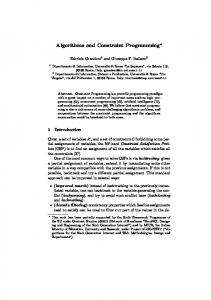
Figure 1: Examples of product tree structures.

Constraint Programming (CP) method is a relatively new technique. It has been identified as a strategic direction and dominant form for the industrial application of production planning and scheduling [10, 11]. It has been proved to be effective in dealing with combined optimization problems because of its broad representational scope and generally applicable solving algorithm. CP was originally developed to solve constraint satisfaction problem (CSP) to find a value for each variable where constraints specify that some subsets of values cannot be used together. And it has been extended to constraint optimized problem (COP) which adds an objective function (such as cost). The optimized solution is achieved by solving a CSP in which the objective function of the problem is rewritten as a constraint that forces it to be equal to a new value. Constraint-based scheduling is the discipline that studies how to solve the scheduling problems by using CP. It is analyzed and discussed by using theory and examples including how objectives, decisionvariables, and penalty factors are handled in the literature [12]. The research group also presents an integrated approach that uses the complementary strengths of MILP and CP for solving the combined planning and scheduling problem within an APS system as part of the core optimization engine [13]. A constraint programming technique and a new genetic algorithm are proposed to solve a preemptive and nonpreemptive scheduling model as one of the advanced scheduling problems in the literature [14]. The experiment results show that the proposed method is effective. However, it is only applied to job-shop scheduling problems under a single machine. The literature [15] concentrates on building a constraint programming model in a flexible manufacturing system, but the solving algorithm is not discussed. In this paper, a constraint programming method for advanced planning and scheduling system with multilevel structured products is presented. The constraint programming model with multilevel structured products was proposed with the consideration of precedence constraints, capacity constraints, release time, and due date. The solving process for the COP combines constraint programming method with branch and bound algorithm. The constraint propagation and branching strategy are discussed to deal with

CSP. This paper is organized as follows. Section 2 describes the problem of APS that we studied; Section 3 introduces the constraint programming model and the solving algorithm in detail; a computational study is given to illustrate the effectiveness of this model and algorithm in Section 4; some conclusions and further research direction will be given in Section 5.

2. Problem Description The advanced planning and scheduling problem defined in this paper is similar to the situation in the literature [6] which deals with it by a mixed integer programming (MIP) method. The products considered in this system have multilevel structures. The product tree structure (bill of material) defines the precedence constraints in scheduling problems (Figure 1). The information in the circle gives the operation number and its processing machines. The number on the arrows shows the quantity of material needed for a final product (the default number is 1). For example, the final product five (with the assembly 5-6) is composed of one subassembly (5-3) and two components (5-4 and 5-5). Meanwhile, the subassembly (5-3) is made up of components (5-1 and 5-2). This multilevel structure is typical in industry production and is often more complex than this example. Assume that a production system contains 𝑀 machines and 𝐼 products. Every product 𝑖 has 𝑛𝑖 operations. Every operation task(𝑖, 𝑗) can be processed on a dedicated machine. An optimal schedule for the products should be found to minimize the total cost including tardy cost and early cost. Some conditions are assumed to reduce the complexity of the problem. The product tree structure, release time, and due date are known in advance and similarly for processing time of operations. A lot-for-lot strategy is adopted for making products, while the setup times are negligible.

3. Constraint Programming Approach The classic definition of a constraint satisfaction problem (CSP) is as follows. A CSP is a triple 𝑃 = (𝑋, 𝐷, 𝐶), where 𝑋 is an 𝑛-tuple of variables 𝑋 = (𝑥1 , 𝑥2 , . . . , 𝑥𝑛 ), 𝐷 is a

Discrete Dynamics in Nature and Society corresponding 𝑛-tuple of domains 𝐷 = (𝐷1 , 𝐷2 , . . . , 𝐷𝑛 ) such that 𝑥𝑖 ∈ 𝐷𝑖 , and 𝐶 is a 𝑡-tuple of constraints 𝐶 = (𝐶1 , 𝐶2 , . . . . , C𝑡 ). A solution to the CSP is an 𝑛-tuple 𝐴 = {𝑎1 , 𝑎2 , . . . . , 𝑎𝑛 }, where 𝑎𝑖 ∈ 𝐷𝑖 and each 𝐶𝑗 is satisfied. The algorithm for solving constraint model can be classified into two categories: inference and search [16]. Inference techniques can eliminate large subspaces by local constraint propagation method. Search systematically explores solution, often eliminating subspaces with a single failure. These two basic strategies are usually combined in most applications. CSP provides a feasible solution satisfying all the constraints. But in real life, we try to find an optimal or relatively better solution with a definite objective such as the minimization of the cost or time. As a result, the emergency of the constraint optimization problem (COP) is extended from CSP. The solving algorithm for COP is based on CSP. The domain of the objective function value is defined by the lower bound (LB) and upper bound (UB) and it is gradually restricted with the calculation process. The objective function is rewritten as a constraint which forces it to be equal to (or less than, or more than) a new value (generally, it is a liner relation with LB and UB). Then the COP is transferred to solve CSP iteratively. Once a feasible solution is found, the LB or the UB is changed and the additional constraint for the objective is restricted. The search terminates when LB equals UB or all the nodes are fathomed. 3.1. The Constraint Programming Model. In order to build the APS constraint programming model, the following notations are used to describe the problem: 𝑖: product index

3 𝑙𝑖 : tardy days of product 𝑖 (real) 𝐸𝑖 : early days of product 𝑖 (integer) 𝐿 𝑖 : tardy days of product 𝑖 (integer). The variable of the constraint model for advanced planning and scheduling problem is the start time of each operation task(𝑖, 𝑗).start. The variable task(𝑖, 𝑗).duration and task(𝑖, 𝑗).end, respectively, denote duration time and end time of operation task(𝑖, 𝑗). The equation task(𝑖, 𝑗).start + task(𝑖, 𝑗).duration = task(𝑖, 𝑗).end clarifies their relationship. The problem described in Section 2 can be formulated as the following model: 𝐼

Min

𝑍 = ∑ (𝑇𝐶 ⋅ 𝐿 𝑖 + 𝐸𝐶 ⋅ 𝐸𝑖 )

subject to

Parameters 𝐼: number of products 𝑀: number of machines 𝑁𝑖 : operation number of product 𝑖 task(𝑖, 𝑗): the 𝑗th operation of product 𝑖 𝑞𝑖𝑗 : the quantity of part which task(𝑖, 𝑗) takes 𝑡𝑖𝑗 : the processing tome of the operation task(𝑖, 𝑗) V𝑖 : the quantity of product 𝑖 𝑟𝑖 : the release time of product 𝑖 𝑑𝑖 : the due time of product 𝑖 𝑧𝑖𝑗𝑘 : 1 if the operation task(𝑖, 𝑗) precedes operation task(𝑖, 𝑘), 0 otherwise 𝐻: the effective work time per day TC: cost of tardy products per day per job EC: cost of early products per day per job. Variables 𝐶max : production makespan 𝑒𝑖 : early days of product 𝑖 (real)

∀𝑖, 𝑗

task (𝑖, 𝑗) .start ≥ 𝑟𝑖

task (𝑖, 𝑗) .duration = 𝑡𝑖𝑗 ⋅ 𝑞𝑖𝑗 ⋅ V𝑖 task (𝑖, 𝑛 (𝑖)) .end ≤ 𝐶max

(2) ∀𝑖, 𝑗

∀𝑖,

(3) (4)

task (𝑖, 𝑘) .start + task (𝑖, 𝑘) .duration ≤ task (𝑗, 𝑝) .start or task (𝑗, 𝑝) .start + task (𝑗, 𝑝) .duration ≤ task (𝑖, 𝑘) .start

(5)

∀𝑖, 𝑗, 𝑘, 𝑝 ∈ {𝑖, 𝑗, 𝑘, 𝑝 | task (𝑖, 𝑘) ≠ task (𝑗, 𝑝) ,

𝑚: machine index 𝑗: operation index.

(1)

𝑖=1

𝑅𝐸𝑆 (𝑖, 𝑘) = 𝑅𝐸𝑆 (𝑗, 𝑝)} task (𝑖, 𝑗) .start + task (𝑖, 𝑗) .duration ≤ task (𝑖, 𝑘) .start 𝑖,

𝑗, 𝑘 ∈ {𝑖, 𝑗, 𝑘 | 𝑧𝑖𝑗𝑘 = 1} ,

(6)

𝐶𝑖 − 𝑑𝑖 ≤ 𝑙𝑖 , 𝐻

∀𝑖,

(7)

𝐶𝑖 ≤ 𝑒𝑖 , 𝐻

∀𝑖,

(8)

𝑑𝑖 −

𝐿 𝑖 ≥ 𝑙𝑖

∀𝑖,

(9)

𝐸𝑖 ≥ 𝑒𝑖 − 0.99

∀𝑖,

(10)

𝐿 𝑖 , 𝐸𝑖 , 𝑙𝑖 , 𝑒𝑖 ≥ 0

∀𝑖.

(11)

The objective is to minimize the total cost which includes the early cost and tardy cost. The penalties on tardiness and earliness mean just-in-time (either early or late delivery results in an increase in the cost). The multilevel structure of products is defined by the binary parameter 𝑧𝑖𝑗𝑘 , which can express all the tree structures. Constraint (2) means that the start time of each operation should not be less than the release time of the product. Constraint (3) defines the duration of each operation. Constraint (4) shows that the completion time of

4

Discrete Dynamics in Nature and Society

each product should be less than or equal to the makespan. Constraint (5) implies that if two operations require the same machine, then one cannot start before the end of the other operation. Constraint (6) ensures the precedence constraints based on the product tree structure. Constraints (7) and (8) define the early time and tardy time (real type) of each product. Constraints (9) and (10) convert the value of real type time to integer type because the penalty costs are in the unit of days. Constraint (11) indicates the domain of variables.

Start

Variable selected Branching strategy Scan all the value?

3.2. Solving Approach. The proposed constraint programming model is a COP which can be transferred to CSPs with the addition of an objective function value constraint 𝑍 ⩽ 𝐶.

(12)

We delete the objective function (1) and add constraint (12) to structure a CSP. The optimal solution of the COP can be generated by iteratively solving the CSP and continuously restricting constraint (12). The detailed solving steps can be summarized as follows.

Backtrack Y

N Value selected Y Y Constraint propagation

Conflict?

Step 1. Compute the LB and UB of the objective function 𝑍. Step 2. Add the constraint 𝑍 ⩽ 𝐶, where 𝐶 = (LB + UB)/2 to the CSP.

N

Uninstantiated variable exist?

Step 3. Solve the CSP and set a fixed time cutoff. If a feasible solution 𝑆 is found, the UB is updated to the value of the objective function 𝑍(𝑆). Else, update LB = 𝐶 + 1.

Feasible solution found

Step 4. Repeat Steps 2 and 3, until LB = UB. Initially, the UB of the objective function 𝑍 is calculated by solving the CSP without constraint (12) to find an initial feasible solution 𝑆0 . The UB is set to be equal to the value of 𝑍(𝑆0 ). While the LB of the objective function 𝑍 is calculated by the constraint propagation technique to determine the time window of each operation which will be introduced in Section 3.2.1, LB is formulated as follows: 𝐼

𝐿𝐵𝑧 = 𝑇𝐶 ⋅ ∑ max {0, ⌈ 𝑖=1

𝐼

N

𝐶𝑖 min − 𝑑𝑖 ⌉} 𝐻 (13)

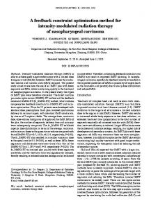
𝐶 + 𝐸𝐶 ⋅ ∑ max {0, ⌈𝑑𝑖 − 𝑖 max − 0.99⌉} , 𝐻 𝑖=1 where 𝐶𝑖 min is equal to the earliest start time of the last operation task(𝑖, 𝑛𝑖 ) plus the processing time of the operation. Correspondingly, 𝐶𝑖 max equals the latest start time of the last operation task(𝑖, 𝑛𝑖 ) plus the processing time of the operation. The symbol ⌈𝑥⌉ is the smallest integer greater than or equal to 𝑥. Since the starting upper bound is often very poor, we reduce the gap by performing a dichotomic search. In this paper, the solving process of CSP in Step 3 is based on a depth-first exploration of the search tree (Figure 2). At each node, a propagation phase is triggered in order to detect possible inconsistencies and reduce the search space. If this phase detects an inconsistency, the algorithm

End

Figure 2: Flow chart of CSP solving process.

backtracks and removes the effects of the previous decision. If no inconsistency is detected, a branching process is applied recursively to the child nodes until a solution is found or until all the search spaces have been explored. So in the next two parts, we will introduce the constraint propagation technique and branching strategies which directly influence the search speed. 3.2.1. Constraint Propagation. The propagation phase is fundamental to reduce the size of the search space and to avoid exploring an exponential size space. The constraint propagation could be based on time or resources. Usually, timetable method uses time window to express the constraints when using constraint propagation based on time. The time window of the start time of an operation task(𝑖, 𝑗) is [task(𝑖, 𝑗).est, task(𝑖, 𝑗).lst], in which task(𝑖, 𝑗).est means the earliest start time and task(𝑖, 𝑗).lst means the latest start time. The time window will be tightened during the constraint propagation process. Once an operation’s time window is


5 Table 1: Product information.

Products 1 2 3 4 5

(V𝑖 , 𝑟𝑖 , 𝑑𝑖 ) (8, 0, 2) (4, 20, 5) (6, 10, 4) (8, 50, 3) (6, 0, 5)

O1 5 5 4 5 3

O2 4 10 5 4 5

changed, then the time window of succeeding and preceding operations will be also changed. The constraint propagation rule for timetable is as follows: task (𝑖, 𝑗) .est = 𝑟𝑖

∀𝑖, 𝑗 ∈ {𝑖, 𝑗 | 𝑧𝑖𝑘𝑗 = 0 ∀𝑘}

(14)

task (𝑖, 𝑘) .est = task (𝑖, 𝑗) .est + task (𝑖, 𝑗) .duration ∀𝑖, 𝑗, 𝑘 ∈ {𝑖, 𝑗, 𝑘 | 𝑧𝑖𝑗𝑘 = 1} task (𝑖, 𝑗) .lst = 𝐶max (𝑆0 ) − task (𝑖, 𝑗) .duration ∀𝑖, 𝑗 ∈ {𝑖, 𝑗 | 𝑧𝑖𝑗𝑘 = 0 ∀𝑘}

(15)

(16)

task (𝑖, 𝑗) .lst = task (𝑖, 𝑘) .lst − task (𝑖, 𝑘) .duration ∀𝑖, 𝑗, 𝑘 ∈ {𝑖, 𝑗, 𝑘 | 𝑧𝑖𝑗𝑘 = 1} .

(17)

The earliest start time of each operation can be updated by formulae (14) and (15). Formula (14) is defined for the start operations without any operation preceding them. The earliest start time of succeeding operation is updated based on formulae (15) accompanied with the change of the preceding operations. Correspondingly, the latest start time of each operation can be updated by formulae (16) and (17). Formula (16) is defined for the last operations without any operation succeeding it. The latest start time of preceding operation is updated based on formula (17) accompanied with the change of the succeeding operations. 3.2.2. Branching Strategy. The earliest search method used in CP algorithm is the generate-and-test (GT) algorithm. Its efficiency is poor because of noninformed generator and late discovery of inconsistencies, and consequently the backtracking (BT) algorithm was put forward. Backtrack is the fundamental “complete” search method for constraint satisfaction problems. Basic backtracking search builds up a partial solution by choosing values for variables until it reaches a dead end, where the partial solution cannot be consistently extended. Several branching strategies have been proposed for the standard job-shop problem [17]. The branching strategy determines the shape of the search tree which directly influences the search speed. In this part, we will consider three heuristic branching strategies. Strategy 1 (binary constraint heuristic): it creates a binary search tree by branching on the two possibilities defined by a disjunction. Constraint (5) defines two possibilities. Assuming two operations 𝑜𝑖𝑘 and 𝑜𝑗𝑝 share the same machine 𝑚, the constraint task(𝑖, 𝑘).start + task(𝑖, 𝑘).duration ≤

O3 2 3 5 1 6

O4 4 / 10 6 6

O5 / / 5 1 5

O6 / / / 2 5

task(𝑗, 𝑝).start is posted to one branch and the constraint task(𝑗, 𝑝).start + task(𝑗, 𝑝).duration ≤ task(𝑖, 𝑘).start corresponds to another branch. Strategy 2 (variable-based heuristic): we use variable ordering heuristic to select the variable with the smallest domain size. The variables in the constraint model are the start times of each operation. The domain of variable is in the interval of the earliest start time and the latest start time. We select the variable with the smallest domain size and set the value with ascending order. Strategy 3 (task-based heuristic): it consists of the definition of a task selection strategy and a value selection heuristic for the task start times. We select the task with the smallest latest completion time and choose the value with descending order.

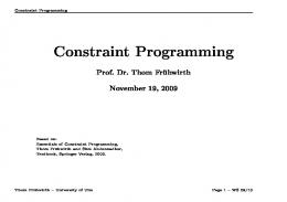
4. Computational Study To illustrate the proposed CP method for advanced planning and scheduling, a simple example is given below which involves five types of products and five types of machines. Figure 1 gives the representation of the product tree structures which shows the processing machines. Table 1 provides more information about these products. A product 𝑖 is described by the triplet (V𝑖 , 𝑟𝑖 , 𝑑𝑖 ), where V𝑖 is the demand quantity, 𝑟𝑖 is the release time, and 𝑑𝑖 is the due date. The processing time of operation task(𝑖, 𝑗) is also shown in this table. The cost of tardiness and earliness is 25 per day and 5 per day. The effective work time is 80 per day. The example model was solved by an OR-optimization software tool called Xpress-MP with 2.53 GHz CPU and 4 GB RAM. The Gantt chart is shown in Figure 3 (we add a virtual machine to allocate the virtual tasks). The makespan is 392. Product 4 is delayed for two days. The optimized total cost is 50. The benchmark does not exist for this problem because it considers all the product tree structures, not only job-shop type. As a result, we generate the testing problems based on the simple example. We extend the data set to three types of problems with different number of products, maximum number of operations, and number of machines (Table 2). Each type contains three instances. Instances a-1 to a-3 are of type 5∗6∗5 (small instances). Instances b-1 to b-3 are of type 10∗6∗5 (medium instances). Instances c-1 to c-3 are of type 5∗21∗5 (large instances). The MIP and CP models are, respectively, solved by Xpress-mmxprs and Xpress-Kalis modules. Table 3 shows the size of the CP and MIP models in terms of the number of variables and constraints according to the above problem

6


Figure 3: Gantt chart of this example. Table 2: Data set. Problem type a b c

No. of products 5 10 5

Max. no. of operations 6 6 21

No. of machines 5 5 5

Table 3: Comparison of CP and MIP models. Instance a-1 a-2 a-3 b-1 b-2 b-3 c-1 c-2 c-3

CP IP No. of variables No. of constraints CPU time (s) Objective No. of variables No. of constraints CPU time (s) Objective 0.1 50 0.2 50 182 539 182 301 0.1 75 0.2 75 0.1 150 0.1 150 0.5 50 37.4 50 337 1964 657 1190 1000+ 75 1000+ 75 3.6 125 1000+ 175 16.5 75 44.4 75 407 13937 4693 9188 5.7 125 1000+ 125 1000+ 300 1000+ 275

The instance results in bold are proved to be optimal.

Table 4: Comparison of the search results of three branching strategies. Problem type a-1 a-2 a-3 b-1 b-2 b-3 c-1 c-2 c-3

1 Computation time (s) 0.05 0.02 0.03 0.488 1000+ 3.596 16.529 5.712 1000+

Backtracks 1166 492 798 5369 100000+ 12359 16522 10636 100000+

Branch strategy 2 Computation time (s) Backtracks 0.122 3601 0.08 1762 0.099 2499 0.897 7354 1000+ 100000+ 5.691 17316 26.253 56329 1000 100000+ 1000 100000+

3 Computation time (s) 0.132 0.09 0.112 10.023 1000+ 1000+ 46.639 36.952 1000+

Backtracks 3601 1862 2499 39392 100000+ 100000+ 92853 89352 100000+

Discrete Dynamics in Nature and Society instances. The MIP models contain a noticeably larger number of variables in all problems than the CP models, while the number of constraints is less than in the CP models. The computation time and the objective value are also shown in this table. It should be also noted that when the problem size is large, the solving time for MIP is increased fast and cannot even get the optimal solution in acceptable time. The instance results in bold are proved to be optimal. The maximum computation time is set to be 1000 s. The CP method gets 7 optimal solutions in 9 instances, while the MIP method only gets 5. The computation time of CP method (strategy 1) is apparently less than that of the MIP method. The branching strategies are also compared in our computational study. The computation time and backtrack iterations are shown in Table 4. It is obviously shown that branching strategy 1 is superior to other strategies in terms of high computation speed and less backtrack times.

5. Conclusion and Future Work We have proposed a constraint programming approach to solve the advanced planning and scheduling problem with multilevel structured products. The cooperation of constraint programming method and branch and bound algorithm is applied to deal with the CP model. And it is proved to be more effective than the MIP model. Moreover, three branching strategies for constraint model are compared. The results have shown that the performance of binary constraint branching strategy is better. This study shows that constraint programming is effective for advanced planning and scheduling problem. Although we have considered all the types of product structures, there still are some conditions we havenot taken into consideration, such as setup time and alternative operations [18]. In our future research, we will build a more comprehensive model closer to the real-life production and design a hybrid algorithm to solve it.

Conflict of Interests The authors declare that there is no conflict of interests regarding the publication of the article.

Acknowledgments This work has been supported by Shanghai Excellent Young Teachers Program (shu11008), the Innovation Found Project of Shanghai University (sdcx2012015), and Natural Science Foundation of Zhejiang (Y6110045).

References [1] K. Sheikh, Manufacturing Resource Planning (MPR II) with an Introduction to ERP, SCM, and MRP, McGraw-Hill, New York, NY, USA, 2003. [2] Advanced Planning and Scheduling in High Tech industry. A Eyeon white paper.

7 [3] H. Stadtlere and C. Kilger, Supply Chain Management and Advanced Planning: Concepts, Models, Software and Case Studies, Springer, Berlin, Germany, 3rd edition, 2005. [4] L.-C. Kung and C.-C. Chern, “Heuristic factory planning algorithm for advanced planning and scheduling,” Computers and Operations Research, vol. 36, no. 9, pp. 2513–2530, 2009. [5] C. Moon, J. S. Kim, and M. Gen, “Advanced planning and scheduling based on precedence and resource constraints for eplant chains,” International Journal of Production Research, vol. 42, no. 15, pp. 2941–2954, 2004. [6] K. J. Chen and P. Ji, “A mixed integer programming model for advanced planning and scheduling (APS),” European Journal of Operational Research, vol. 181, no. 1, pp. 515–522, 2007. ¨ ¨ ¨ urk, “A note on ‘A [7] A. Ornek, S. Ozpeynirci, and C. Ozt¨ mixed integer programming model for advanced planning and scheduling (APS)’,” European Journal of Operational Research, vol. 203, no. 3, pp. 784–785, 2010. ¨ urk and A. M. Ornek, “Operational extended model [8] C. Ozt¨ formulations for advanced planning and scheduling systems,” Applied Mathematical Modelling, vol. 38, no. 1, pp. 181–195, 2014. [9] S. Kreipl and M. Pinedo, “Planning and scheduling in supply chains: an overview of issues in practice,” Production and Operations Management, vol. 13, no. 1, pp. 77–92, 2004. [10] Y. Chen, Z. Guan, Y. Peng, X. Shao, and M. Hasseb, “Technology and system of constraint programming for industry production scheduling. Part I: a brief survey and potential directions,” Frontiers of Mechanical Engineering in China, vol. 5, no. 4, pp. 455–464, 2010. [11] S. Topaloglu, L. Salum, and A. A. Supciller, “Rule-based modeling and constraint programming based solution of the assembly line balancing problem,” Expert Systems with Applications, vol. 39, no. 3, pp. 3484–3493, 2012. [12] H.-H. Hvolby and K. Steger-Jensen, “Technical and industrial issues of advanced planning and scheduling (APS) systems,” Computers in Industry, vol. 61, no. 9, pp. 845–851, 2010. [13] K. Steger-Jensen, H.-H. Hvolby, P. Nielsen, and I. Nielsen, “Advanced planning and scheduling technology,” Production Planning and Control, vol. 22, no. 8, pp. 800–808, 2011. [14] Y.-S. Yun and M. Gen, “Advanced scheduling problem using constraint programming techniques in SCM environment,” Computers and Industrial Engineering, vol. 43, no. 1-2, pp. 213– 229, 2002. [15] L. J. Zeballos, O. D. Quiroga, and G. P. Henning, “A constraint programming model for the scheduling of flexible manufacturing systems with machine and tool limitations,” Engineering Applications of Artificial Intelligence, vol. 23, no. 2, pp. 229–248, 2010. [16] F. Rossi and P. T. Walsh, Handbook of Constraint Programming, Elsevier, Amsterdam, The Netherlands, 2006. [17] A. S. Jain and S. Meeran, “Deterministic job-shop scheduling: past, present and future,” European Journal of Operational Research, vol. 113, no. 2, pp. 390–434, 1999. [18] C. Artigues and D. Feillet, “A branch and bound method for the job-shop problem with sequence-dependent setup times,” Annals of Operations Research, vol. 159, pp. 135–159, 2008.

Advances in

Operations Research Hindawi Publishing Corporation http://www.hindawi.com

Volume 2014

Advances in

Decision Sciences Hindawi Publishing Corporation http://www.hindawi.com

Volume 2014

Journal of

Applied Mathematics

Algebra

Hindawi Publishing Corporation http://www.hindawi.com


Volume 2014

Journal of

Probability and Statistics Volume 2014

The Scientific World Journal Hindawi Publishing Corporation http://www.hindawi.com


Volume 2014

International Journal of

Differential Equations Hindawi Publishing Corporation http://www.hindawi.com

Volume 2014

Volume 2014

Submit your manuscripts at http://www.hindawi.com International Journal of

Advances in

Combinatorics Hindawi Publishing Corporation http://www.hindawi.com

Mathematical Physics Hindawi Publishing Corporation http://www.hindawi.com

Volume 2014

Journal of

Complex Analysis Hindawi Publishing Corporation http://www.hindawi.com

Volume 2014

International Journal of Mathematics and Mathematical Sciences

Mathematical Problems in Engineering

Journal of

Mathematics Hindawi Publishing Corporation http://www.hindawi.com

Volume 2014


Volume 2014

Volume 2014


Volume 2014

Discrete Mathematics

Journal of

Volume 2014



Journal of

Function Spaces Hindawi Publishing Corporation http://www.hindawi.com

Abstract and Applied Analysis

Volume 2014


Volume 2014


Volume 2014

International Journal of

Journal of

Stochastic Analysis

Optimization



Volume 2014

Volume 2014