Using Constraint Programming for Reconfiguration

Using Constraint Programming for Reconfiguration of Electrical Power Distribution Networks ? Juan Francisco D´ıaz2 , Gustavo Gutierrez1 , Carlos Alberto Olarte1 , and Camilo Rueda1 1

2

Pontificia Universidad Javeriana, Cali, Colombia, {crueda,caolarte,ggutierrez}@atlas.puj.edu.co Universidad del Valle, Cali, Colombia [email protected]

Summary. The problem of reconfiguring power distribution system to reduce power losses has been extensively studied because of its significant economic impact. A variety of approximation computational models have recently been proposed. We describe a constraint programming model for this problem, using the MOzArt system. To handle real world reconfiguration systems we implemented and integrated into MOzArt an efficient constraint propagation system for the real numbers. We show how the CP approach leads to a simpler model and allows more flexible control of reconfiguration parameters. We analyze the performance of our system in canonical distribution networks of up to 60 nodes. We describe how the adaptability of the MOzArt search engine allows defining effective strategies for tackling a real distribution system reconfiguration of around 600 nodes.

1 Introduction The purpose of an electric power distribution system is to deliver power to customers. The energy source in this system is a power transformer directly connected to a set of feeders. Each feeder acts as the energy supplier for a given section of the distribution system. Energy from the feeders reach customers through a network of nodes linked by branches (transmission lines). Some of the branches have switches that can be opened (resp. close) to interrupt (resp. allow) the current flow. The topology of lines interconnecting customers to feeders form a mesh network in which radiality must be guaranteed (i.e. there cannot be a path connecting any two different feeders) while ensuring power delivery to all users ? This work was partially supported by the Colombian Institute for Science and Technology Development (Colciencias) under the CRISOL project (Contract No.298-2002)

2

D´ıaz J. et al.

(Service Continuity). Radial networks simplify overcurrent protections in the feeders. A power distribution network usually has to be reconfigured (i.e. the state of some switches changed) from time to time for two reasons: 1) to restore power to customers following a fault and 2) in order to minimize or reduce power losses induced by the resistance and the current in branches. Although similarities exist between reconfiguration strategies in both cases we confine ourselves in this paper to reconfiguration to reduce power losses. When a network is reconfigured it is typically the case that some nodes that were previously connected by a path of branches to a given feeder, connect to a different feeder in the new configuration. For this reason the problem is sometimes referred to as feeder reconfiguration. Customer power loads vary with time of day and day of the week. Each feeder serves a different mix of residential, commercial and industrial loads (i.e. amount of power requested), and each type of load has different time profiles. Consequently, the load pattern on each feeder varies constantly. To keep losses to a minimum in these changing situations feeders must be reconfigured with a frequency that usually depends on the degree of automation available for switch control. The power distribution system should in principle be operated with minimum losses and satisfying different types of constraints: • All customers must be served (i.e. every node in the network should be connected to a feeder) • Radial configuration must be maintained. • Current in lines and transformers should lay within given capacity limits. • Voltage drops limits should be obeyed. For reasons including poor line maintenance, ill planned system growth policies or the presence of unauthorized connections, in developing countries losses in power distribution systems are very high ([3]). Moreover, switch control is usually done manually which means that the number of switching operations performed in reconfiguration must be constrained. Finding (not necessarily optimal) distribution network configurations reducing losses and respecting switching constraints can thus have a significant economic impact. Two main strategies have been previously used for power losses reduction by reconfiguration: 1) start with a feasible (i.e. radial) solution, select a tie switch (the ones linking two feeder circuits) to close (thus forming a loop) and then select a line switch to open to restore radiality ([4]), and 2) start with all tie switches closed (thus forming “weak” loops) and then opening selected switches one by one until radiality is restored ([14]). In both strategies computing losses of each trial configuration entails determining current values in the network by a process called load flow computation. Known values in this computation are essentially customer loads and resistance of network branches. Other electrical values have to be calculated. The process starts with an estimate of voltages and use electrical laws to determine currents.

CRE2

3

These in turn serve to refine the initial guesses. The process iterates until computation of electrical parameters stabilizes. We can thus identify two distinct processes in reconfiguration: selecting a switch to open or close (a combinatorial number of boolean possibilities) and performing load flow computation (calculations over the complex numbers). This constitute a hybrid combinatorial optimization problem. Solutions proposed recently (simulated annealing [10], expert systems [16], tabu search [7]) usually employ approximation techniques to avoid generating (and performing load flow computation of) a combinatorial number of configurations, by focusing search to a small subset of “promising” configurations. In [5, 6] a system (called PLANET) performing power network reconfiguration is presented. This system, based on the constraint language CHIP, aims at finding an optimal maintenance schedule. Since maintenance involves isolating a section of the network, reconfiguration has to be performed to ensure that customers serviced through that section are kept energized (or to minimize those that are not, when full service is not possible). Load flow must also be done to compute fundamental electrical values of the reconfigured network so as to ensure operating constraints. CRE2 , the application implementing the approach presented in this paper, differs from this system in two important ways. First, in its purpose since CRE2 does not address optimal maintenance scheduling, whereas PLANET does not address minimizing power losses. Second, in their technological choices: in CRE2 all computations including load flow, are performed using constraint programming (CP) technology (a real intervals constraint system was developed for load flow). In PLANET, an electric library, written in C, is used for computing load flow and also for reconfiguring (using the heuristic approach in ([14]). The main contribution of this paper is to show that constraint programming can effectively be used both for load flow computation and for reconfiguration. Moreover, we show how the interaction of this two processes modeled in CP can be used to significantly prune the search tree. Implemented in MOzArt ([15], www.mozart-oz.org), our model has been tested successfully in canonical reconfiguration problems of networks up to 60 nodes. To compute load flow we had to implement for MOzArt a new efficient constraint propagation system over the real numbers, based on the interval arithmetic package in [9]. We used the modularity and extension facilities of MOzArt to effectively couple these constraint propagators to the existing finite domain system and also to build into the labeling process strategies better suited to the reconfiguration problem. While our approach is arguably less efficient than some existing approximation schemes, we think using CP provides definite advantages: 1) all electrical and operational power system constraints are always satisfied, 2) provides a simpler computational model, directly related to fundamental electric laws of the system, 3) allows more flexible parameter control, such as maximum number of switching operations and 4) leaves more room to introduction of additional operational constraints or search control strategies.

4

D´ıaz J. et al.

Our research group is interested in studying the application of CP techniques, particularly the MOzArt system, to real world problems. We are currently adapting this implementation to run a losses reduction reconfiguration of a power system network of around 600 nodes in the southern region of Colombia. In section 3 we formally define the reconfiguration problem and describe a constraint model for solving it. In section 4, we analyze the results of running the implementation of this model in two canonical power distribution networks. Finally, sections 5 and 6 are devoted to stating our considerations on the strong and weak points of using CP for this problem and the line of works we plan to pursue.

2 XRI: A Constraints System over Real Intervals XRI is an implementation of a real intervals constraint system for MOzArt . This implementation is an extension of the Real Interval module (RI) implemented by Tobias M¨ ueller ([12]) and distributed as a contribution with the MOzArt sources. The XRI module provides constraint propagators for real intervals relations and a general customizable distribution procedure for real intervals domains. In the following we describe the foundations of our module implementation (interval arithmetic, interval constraints and hull consistency) and its main features (real intervals domains, propagators and distribution). 2.1 Interval Arithmetic and Constraints Interval arithmetic aims at bounding numeric errors appearing when doing calculations with the classical representation of real numbers as floating-point numbers. A closed interval [l, u], with l, u ∈ R can be regarded either as the set of real numbers {r | l ≤ r ≤ u}, or as an approximation of some real number laying within that set. Instead of using a single floating-point number to approximate a real, interval arithmetic encloses the real number within a closed interval having (in general) floating-point bounds. Different intervals can thus approximate the same real number. When the width of the interval is sufficiently small (i.e. the approximation conforms to a desired precision), the interval is said to represent the real number. Any function (arithmetic operation) f over the real numbers can be extended to a function F over intervals by F (I) = outerI ({r | ∃v. v ∈ I ∧ f (v) = r}), where outerI (S) denotes an interval enclosing all values in the set S. It is in general desirable to have the smallest such interval.

CRE2

5

Similarly, any relation over the real numbers can be extended to an interval relation. A cartesian product of intervals, B = I1 × ... × In is called a Box. A relation c(x1 , ..., xn ) over the reals (i.e. a set of tuples) is extended to a relation over intervals: C(I1 , ..., In ) = outerB ({(r1 , ..., rn ) | r ∈ I1 , ..., rn ∈ In ∧ c(r1 , ..., rn )}, where outerB (S) is a box enclosing the set of tuples S. A key issue in interval arithmetic is how to define outer so that tight intervals are obtained. For basic arithmetic functions this can be achieved by simple operations on the bounds of the intervals involved. For example, [l1 , u1 ] + [l2 , u2 ] = [l1 + l2 , u1 + u2 ], [l1 , u1 ] × [l2 , u2 ] = [min(l1 × l2 , l1 × u2 , u1 × l2 , u1 × u2 ), max(l1 × l2 , l1 × u2 , u1 × l2 , u1 × u2 )] A problem is that these operations do not obey the usual algebraic properties (e.g. distributive laws). This means that equivalent arithmetic expressions do not lead to equivalence of their interval extension counterparts. The practical consequence of this fact is that the width of the interval computed by outer might depend on the form a particular expression takes (see [13] for a through discussion of these issues). Section 2.2 describes a way to avoid this problem in some particular cases. In [9] an interval arithmetic system is presented, using function and relation extensions with the properties of correctness (operating on any values in the argument intervals always gives a value belonging to the result interval), totality (interval operations are defined on all intervals), closeness (interval operations return intervals), optimization (interval results are not wider than necessary) and efficiency. It is also shown how to implement basic arithmetic operators extensions over intervals (such as + and ×), on a computer meeting the IEEE754-Standard for floating-point arithmetic. The term interval constraint denotes a constraint in which variables are associated to intervals. In our implementation this interval (the domain of the variable) represents in reality the set of all its subintervals. The value of a variable is thus always an interval (a sufficiently narrow one). XRI is an implementation of efficient techniques for solving sets of interval constraints, integrated as constraint propagators of MOzArt . Research in this area (see for example [2]) is devoted to finding correct and (near) optimal interval propagation techniques that can be efficiently implemented. These techniques are known as narrowing algorithms whereas propagators for constraints are called constraint narrowing operators. A constraint narrowing operator transforms the domains of those variables involved in it into tighter intervals such that: • Result intervals are always included in the original ones ( contractance property).

6

D´ıaz J. et al.

• All values in the original intervals verifying the associated constraint of the narrowing operator, belong to the result intervals ( soundness or correctness). • The subset interval relation is conserved by the transformation (monotonicity). Well known examples of constraint narrowing operators are Hull and Box Consistency (see [2]) and kB−Consistency Operators (see [11] ). The current version of XRI contains an efficient implementation of Hull consistency known as HC4 (see next section). 2.2 HC4 A major problem of interval arithmetic is the overestimation of results. As mentioned before, this might be a consequence of the form the arithmetic expression takes. For instance, extending the function f (x) = x2 − 2x + 1 on the interval x = [−1, 3] we get F ([−1, 3]) = [−4, 4]. If the function is equivalently written f (x) = (x − 1)2 , then we get F ([−1, 3]) = [0, 4]. This is the so-called data dependency problem: interval operations work independently on each occurrence of a variable, i.e. they consider the above expression as x21 − 2x2 + 1 and then extend it with x1 = [−1, 3], x2 = [−1, 3]. A related problem occurs when constraint propagators for arithmetic equations are defined over a fixed number of variables. For example, if a propagator for interval equations of the form X + Y = Z expects three variables, then an interval equation like X + Y + Z = W must be split into equations T1 = X + Y, T2 = T1 + Z, T2 = W using two new “temporal” variables. Since interval values for these are not known, information on the fact that all variables in the original equation are related is lost. Moreover, the constraint system would have to launch three propagators instead of just one. An efficient hull consistency algorithm called HC4 was proposed by Benhamou in [2]. Input to HC4 is a constraint in “user form” (i.e. without decomposing it in several equations). The algorithm efficiently computes an interval extension of the equation, narrowing intervals of the variables involved. In HC4 the input equation is represented as an attribute tree where the root node is a p-ary relation symbol and terms in the equation form subtrees rooted at nodes containing either a variable, a constant or an operation symbol. Algorithm HC4 works in two phases called “forward evaluation” and “backward propagation”. The forward phase is a tree traversal going from the leaves to the root, evaluating at each node the natural interval extension of that subterm of the constraint. The backward phase traverses the tree from the root to the leaves projecting on each node the effects of interval narrowings already performed on its parent node. In the ”backward propagation phase” an interval may become empty. When this happens the constraint is inconsistent w.r.t. the initial domains. In the XRI module, the user can define a precision for each variable. This value is used in propagators to control the minimum narrowing considered

CRE2

7

significant. If narrowing is less than that, HC4 does not change the intervals. Addition of this control is a consequence of a pathological behavior we observed in some problems: the algorithm may sometimes narrow an interval, say, by one floating point value causing the HC4 propagator to be triggered again to narrow an additional float, and so on. The rationale then is to let in this case other propagators narrow in a more significant way the intervals involved. We implement HC4 as a MOzArt propagator. It uses the MOzArt propagator control, garbage collection and computation space cloning. This guarantees that it is triggered when the interval domain of any of its associated variables is changed by some other propagator (either basic or HC4). The user defines a HC4 propagator by a procedure call whose argument is the constraint written in prefix form. For example, {XRI.hc4 eq(plus(square(X)Y 1.0) plus(times(2.0 X)W ))} sets up a propagator for equation x2 + y + 1.0 = 2.0x + w Other than equality(eq), relational operators < (lt),>(gt),≤(leq) are supported by XRI.hc4, as well as several arithmetic and trigonometric functions. 2.3 XRI Variables and Propagators As said before, the domain of a XRI variable is an interval with floating-point bounds, denoting the set of all its subintervals. Interval bounds are updated via the application of a set of hull-consistency based propagators. A variable is determined when the width of the interval is less than a given precision. In XRI, precision can be defined globally or assigned locally to each variable. A failure occurs when the domain of a variable becomes empty, i.e when its interval lower bound is greater than the upper bound. As is usual in constraints systems, computational agents (called propagators) in XRI work to enforce relations (constraints) among variables in the store. The XRI module offers two kinds of propagators: basic propagators enforcing basic arithmetic constraints, and the HC4 propagator described above. Basic propagators implement interval extensions of basic arithmetic and trigonometric constraints. A constraint is asserted by a MOzArt procedure call of the form {XRI.op X Y Z}, where suffix “op” is an appropriate operator. For example, {XRI.plus X Y Z} asserts constraint X ⊕ Y = Z, where X, Y and Z are interval variables and ⊕ denotes interval addition. Constraint Z = Y X can of course be asserted with the same propagator by invoking {XRI.plus X Z Y}). Floating point operations performed by arithmetic constraints propagators comply with the IEEE754-standard. XRI also offers other propagators with floating point operations not covered by the IEEE754-standard, in particular for trigonometric and logarithmic constraints.

8

D´ıaz J. et al.

2.4 XRI Distribution Distribution is the process used in most constraints systems to guarantee completeness. The XRI module provides a customizable distributor of interval variables similar to the one provided in the MOzArt finite domains module. In the XRI distributor the user can specify the order in which variables are to be distributed, the order in which values should be tested (e.g. try first the lower half interval), and can also supply a procedure to be run when a computation space becomes stable (i.e. when no propagator is active). Well known strategies are provided by default: first-fail, naive and split-upper. The first-fail strategy tells the distributor to select the variable having the smallest domain first and to test first the lower half of the interval. A naive strategy distributes the list of variables in the order they were originally supplied to the distributor, also checking first the lower half of the interval. The split-upper strategy tries the upper half of the interval first.

3 CRE2 : A power distribution system reconfigurator CRE2 is an application written in MOzArt for reconfiguring power distribution networks for power losses reduction. It includes two distinct interacting processes: load flow computation (finding values for electrical variables) using the XRI constraint system and reconfiguration (finding new network topologies) using the MOzArt finite domain constraint system (FD). As said before, an electric distribution network consists of a power transformer connected to a set of feeders, each supplying power to a subnetwork of nodes. Some of the nodes represent customer connected to the distribution system. These nodes have associated active (P ) and reactive (Q) loads. Active loads are the amount of power (measured in watts) actually consumed by the user whereas reactive power (measured in “volt-amperes-reactive”, or var) is an abstract quantity used to describe the effects of a load which on the average neither supplies nor consumes power. It is known that reactive devices such as inductors and capacitors dissipate zero power, yet the fact that they drop voltage and draw current gives the deceptive impression that they actually do dissipate power. This ”phantom power” is called reactive power. Power losses in a network are highly dependent on both P and Q. Nodes (and feeders) are connected by branches. A resistance R and a reactance X is associated with each branch. In certain branches current flow (or lack thereof) along that branch is controlled by a switch. The load flow problem consists in finding values for all electrical variables involved in the network, given values for P , Q, R and X. These variables include the current along each branch (I), the voltage in each node (V ) and the output current (or load current) generated by the power consumed by each user denoted Iq . Active (Lp = |I|2 × R) and reactive (Lq = |I|2 × X) losses

CRE2

9

along each branch are then computed. Summing the latter for all branches gives the overall power loss of the system. Values found must satisfy both the fundamental electrical laws described in section 3.1 and also the operational constraints listed in section 3.2. 3.1 Electrical constraints Values computed in the load flow process should obey: Ohm law equations (1) on each branch , Kirchoff laws on each node and two equation relating load current w.r.t P and Q. In the following equations, variable Z (impedance) is equal to R + Xi. For each branch with a closed switch in the network, Ohm’s law must hold: ∆V = Z × I

(1)

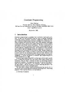
Electrical equations such as 1 can be expressed either in rectangular form (real and imaginary parts) or in polar form (angles and magnitudes). Constraints in polar form require trigonometric propagators whereas those in rectangular form need basic arithmetic propagators. Since the latter can be made stronger and more efficient than the former, CRE2 uses the rectangular representation. Furthermore, magnitude and angle can easily be computed from the rectangular values. Equation 1 can be decomposed into equations 2 and 3; figure 1 shows an MOzArt procedure implementing those equations. V1 .real − V2 .real = I.real × R − I.img × X

(2)

V1 .img − V2 .img = I.real × X + I.img × R

(3)

For each node in the network Kirchoff Law asserts that: X X input branch current = output branch current

(4)

In radial systems the above equation can be simplified to: X input branch current = output branch current + Iq

(5)

where Iq can be computed by: P = V.real × Iq.real + V.img × Iq.img

(6)

Q = V.img × Iq.real − V.real × Iq.img

(7)

10

D´ıaz J. et al.

proc {LOhm InfBranches VarBranches VarNodes EstSw} for I in 1..{Width InfBranches} do Id#N1#N2#R#X#CCR#Ss#Eso = InfBranches.I V1_real = VarNodes.vo_real.N1 V1_img = VarNodes.vo_img.N1 V2_real = VarNodes.vo_real.N2 V2_img = VarNodes.vo_img.N2 I_real = VarBranches.io_real.Id I_img = VarBranches.io_img.Id in if Ss==0 orelse {Nth EstSw I} == 1 then {XRI.hc4 eq(sub(V1_real V2_real) sub(times(I_real R) times(I_img X)))} {XRI.hc4 eq(sub(V1_img V2_img) plus(times(I_real X) times(I_img R)))} end end end Fig. 1. Ohm law procedure

3.2 Reconfiguration procedure The feeder reconfiguration problem can be modeled using finite domains to represent the state of each switch (0 for open, 1 for closed). The target configuration (network topology) must satisfy the following constraints: • Radiality: The number of branches supplying current into a given node must be equal to one • Service Continuity: current must flow to all nodes • Maximum switching operations: limits the number of switches that can be changed • Active losses reduction: active losses in the new topology must be less than in the original network. We implemented a FD procedure enforcing service continuity using the F D.sum propagator (each node has at least one incident closed branch). System radiality is enforced in the load flow procedure by computing the direction of current flow in the network and then verifying that each node has exactly one input current. Finally, the maximum switching operations constraint is implemented using a reified constraint computing the number k of switch changes and asserting a F D.atM ost propagator using k. Our method uses a reconfiguration technique in which switch changes are guided by the goal of balancing power loads among the feeders. For each trial configuration the load flow procedure is invoked to compute its active losses. Configurations in which power losses are not less (by a given amount) than in the original one are rejected.

CRE2

11

Operational Constraints Most reconfiguration methods reported in the literature must verify their solutions against operational constraints. Since CRE2 uses a CP model, operational constraints interact with the search procedure. Some operational constraints are expressed as HC4 equations and can be easily integrated to the load flow procedure itself. For example, we can easily impose operational limits over voltage in nodes and current in branches: • Voltage limit in internal nodes: 1.0 − P vM N O ≤

p Vo .real2 + Vo .img 2

(8)

Asserting that voltage magnitude in each node cannot drop below an operational percentage (P vM N O). • Limit of current in branches: p Io .real2 + Io .img 2 ≤ CCR × (1.0 + P sCP R) (9) Asserting that the percentage of overcurrent in branches (P sCP R) cannot exceed the current limit of the conductor (CCR).

4 Results This section describes the results obtained by running CRE2 on two canonical problems we will refer to as Civanlar (16 nodes, [4]) and Baran (53 nodes, [1]). In both cases a reconfiguration minimizing active losses must be found. All tests were done on an Intel Pentium 4 1.80 GHz computer with 256 of RAM, running Linux Gentoo 1.4 with kernel 2.6.20 and MOzArt system 1.2.5. The Civanlar system consists of 3 circuits (each one starting with a different feeder). Circuits have 5, 6, and 5 nodes, respectively (including the feeders). Any pair of circuits is connect each by a branch containing a switch (initially open). A normalized active losses reduction (0.0054 per unit ) of the initial configuration was found in 142ms using a precision of 10−5 . Computing losses for all feasible reconfigurations achieving some reduction and performing at most four switching operations (see table 1), took 8.30s. In table 1, column “Proposed configurations” specify switches to open and/or close (only four out of seven possible reconfigurations are shown), and column ”% gain” shows the reduction percentage w.r.t the initial active losses. 4.1 Baran case The Baran system consists of 5 circuits having 6,9, 6, 18 and 14 nodes, respectively. Active losses in the original network (0.0013 pu) were computed in 572ms. Not all reconfigurations were searched for due to the huge size of the search tree. Some configurations reducing losses and performing four switching operations at most are summarized in table 2.

12

D´ıaz J. et al.

Active Losses % Gain [p.u] 0.0053 1.85 0.0054 0.00 0.0054 0.00 0.0049 9.25

Proposed reconfigurations Open 4,7 and close 15,16 The initial topology Open 7,13 and close 15,16 Open 7,8 and close 14,15 (Best Configuration)

Table 1. Reconfiguration of Civanlar case Active Losses % Gain [p.u] 0.0012 7.69 0.0011 15.38 0.0010 23.08

Proposed reconfigurations Open 47 and close 53 Open 46 and close 53 Open 32,35,46 and close 51,52,53

Table 2. Reconfiguration of Baran case

5 Conclusions One of the main challenges we faced was to integrate into MOzArt a robust, correct and efficient constraint system for real intervals. Although the XRI module is still being improved, we believe it does provide in its present state good functionality and reasonable performance. As usual in CP, efficiency was strongly dependent on the constraint model used. We initially enforced all electric constraints both in polar and in rectangular form, trying to obtain better interval narrowing by constraint redundancy. We did not obtain the results we expected. We conclude that our propagators for trigonometric constraints are not yet efficient enough to handle real world applications. A redundant constraint that did cause a significant improvement was asserting that the number of closed switches in branches entering a node must be at least one. In this way, no configuration isolating nodes is generated. We have shown that using CP is a real alternative for the problem of reducing power losses by network reconfiguration. Optimal configurations were found in reasonable time for two canonical problems. Moreover, other approaches aim at finding one (hopefully optimal) configuration. In some practical cases, a (not necessarily optimal) configuration reducing losses and satisfying some extra operational constraints (such as number of switch changes) might be a better option. Our CP model easily handles these cases. In addition, CRE2 provide more flexibility, such as the ability to incorporate new load flow models or to add new operational constraints. It is also easy to integrate strategies that have been proved to be effective in some cases. For example, totally meshed networks have minimal losses. A good strategy is then starting with this type of network and open selected switches one by one. This strategy is “free” in our CP model: the distribution strategy simply selects the upper

CRE2

13

value first for switch state (1= a closed switch) and constraints quickly prune non radial networks. Although the computation time of CRE2 on the canonical problems was greater than in other approaches, it has to be considered that our model actually solved a somewhat (more complex) different problem. We assumed every branch in the network had a switch. This, of course, greatly increases the size of the search tree. In real networks only a few number of switches exist. The reason we model the problem in this way is that, for the particular network we have in mind, we would also like to suggest the best places to install a given number of switches, an issue not considered in other approaches. It is clear to us that handling bigger networks requires better distribution strategies than those currently implemented. We have tried some problem domain driven strategies, such as ensuring each time a switch has to be opened to choose the one that better balances loads in the resulting two circuits. For small problems, the potential gains of this strategy are countered by the time spent in computing subnetwork loads. We still lack enough evidence to claim this improves performance significantly in large networks.

6 Future Work We implemented in CRE2 a network of around 600 nodes corresponding to six electric circuits of the power system for the city of Buenaventura in Colombia. We plan to have reconfiguration results in the short term. We plan to pursue CP formulation of related problems in electrical engineering, such as the unit commitment problem and the service restoration problem ([8]).

Acknowledgments We are greatly indebted to Gladys Caicedo and Carlos Lozano, from the GRALTA research group 3 , for pointing the reconfiguration problem to the authors and for many enlightening discussions. We are also grateful to James Ortiz, Janeth Rodr´ıguez and Diana Torres for their patient debugging of the initial implementations. Finally, we would like to thank the anonymous reviewers for their valuable comments for improving this paper.

References 1. M.E. Baran and F.F: Wu. Network reconfiguration in distribution systems for loss reduction and load balancing. IEEE Transactions on Power Delivery, 4(2):1401–1407, April 1989. 3

High Tension Research group, Universidad del Valle

14

D´ıaz J. et al.

2. F. Benhamou, Fr´ederic Goualard, and Laurent Granvilliers. Revising hull and box consistency. In Proceedings of ICLP’99 - MIT Press, pages 230–244, 1999. 3. G. Caicedo. Nueva propuesta en reconfiguracion de alimentadores utilizando programacion con restricciones, 2004. PhD thesis, Universidad del Valle, Cali, Colombia. 4. S. Civanlar, J.J. Grainger, H. Yin, and S.S. Lee. Distribution feeder reconfiguration for loss reduction. IEEE Transactions on Power Delivery, 3(3):1217–1223, July 1988. 5. T. Creemers, L. Ros, J. Riera, C. Ferrarons, J. Roca, and X. Corbella. Constraint-based maintenance scheduling on an electric power-distribution network. In Third International Conference and Exhibition on Practical Applications of Prolog, April 1995. 6. T. Creemers, L. Ros, J. Riera, C. Ferrarons, J. Roca, and X. Corbella. Programacin optima de tareas de mantenimiento y reconfiguracin sobre redes de media tensin. In The Fourth Portuguese-Spanish Conference on Electrical Engineering, July 1995. 7. Y. Fukuyama. Reactive tabu search for distribution load transfer operation. In IEEE PES winter meeting, Singapore, January 2000. 8. Y. Fukuyama and H. D. Chiang. Modern heuristic techniques for combinatorial problem. In Proc. of IEEE FUZZ/IFES conference, Yokohama, March 1995. 9. T. Hickey, Q. Ju, and M. H. Van Emden. Interval arithmetic: From principles to implementation. Journal of the ACM, 48(5):1038–1068, September 2001. 10. Y.J. Jeon, J.Ch. Kim, J.O. Kim, J.R Shin, and K.Y. Lee. An efficient simmulated annealing algorithm for network reconfiguration in large-scale distribution systems. IEEE Transactions on Power Delivery, 17(4):1070–1078, October 2002. 11. O. Lhomme. Consistency techniques for numeric csps. In Proceedings of the 13th IJCAI, IEEE Computer Society Press, pages 232–238, 1993. 12. Tobias M¨ uller. Adding constraint systems to DFKI Oz. In WOz’95, International Workshop on Oz Programming, Institut Dalle Molle d’Intelligence Artificielle Perceptive, Martigny, Switzerland, 29 November–1 December 1995. 13. A. Neumaier. Interval methods for system of equations. Cambridge University Press, 1990. 14. H. Shirmohammadi and W. Hong. Reconfiguration of electric distribution networks for resistive line losses reduction. IEEE Transactions on Power Delivery, 4(2):1492–1498, April 1989. 15. G. Smolka. A foundation for higher-order concurrent constraint programming. In Jean-Pierre Jouannaud, editor, 1st International Conference on Constraints in Computational Logics, Lecture Notes in Computer Science, vol. 845, pages 50–72, M¨ unchen, Germany, September 1994. Springer-Verlag. 16. C.T. Su and C.S Lee. Feeder reconfiguration and capacitor setting for loss reduction of distribution systems. Elect. Power Syst. Res., 58(2):97–102, 2001.