A Constructive and Autonomous Integration Scheme of Low-Cost GPS ...

A Constructive and Autonomous Integration Scheme of Low-Cost GPS/MEMS IMU for Land Vehicular Navigation Applications Kai-Wei Chiang1 , Semah Nassar2, and Naser El-Sheimy2. 1

Department of Geomatics, National Cheng-Kung University No.1, Ta-Hsueh Road, Tainan 701, Taiwan. 2 Mobile Multi-Sensor Systems Research Group Department of Geomatics Engineering, The University of Calgary Calgary, Alberta, CANADA T2N 1N4

Abstract — The integration of GPS and INS provides a system that has superior performance in comparison with either a GPS or an INS stand-alone systems. Most integrated GPS/INS positioning systems have been implemented using Kalman Filter (KF) technique. Although of being widely used, KF has some drawbacks related to computation load, immunity to noise effects and observability. In addition, KF only works well under certain predefined error models and provides accurate estimation of INS errors only during the availability of GPS signal. Upon losing the GPS signals, if the inertial sensor errors do not have an accurate stochastic model, Kalman filter delivers poor prediction of INS errors, and thus a considerable increase in position errors may be observed. The impact of these limitations affects the integrated system positional accuracy during GPS signal outages. Recently, the field of artificial intelligence has been receiving more attention in the development of alternative GPS/INS integration schemes. Therefore, in this paper, an alternative scheme is proposed which implements a Constructive Neural Network (CNN). The proposed scheme has flexible topology when compared to the recently utilized Multi-layer Feed-forward Neural Networks (MFNNs). The topologies of MFNN-based schemes are decided empirically with intensive training efforts and they remain fixed during navigation. In contrast, the proposed CNN scheme can adjust its architecture (i.e. the number of hidden neurons) autonomously during navigation based on the complexity of the problem in hand (i.e. dynamic variations) without the need for human intervention. The proposed scheme is implemented and tested using MEMS IMU data collected in land-vehicle environment. It does not require prior knowledge or empirical trials to implement the proposed architecture since it is able to adjust its architecture “on the fly” based on the complexity of the vehicle dynamic variations. This is a significant improvement compared to the previously developed MFNN scheme that requires extensive empirical trials. In addition, the proposed CNN architecture remains fixed after the final design. The proposed scheme performance is compared to both MFNN and KF during several GPS signal outages. The results of all schemes are then analyzed and discussed.

0-7803-9454-2/06/$20.00/©2006 IEEE

I. INTRODUCTION An integrated navigation system that augments complementary navigation sensors such as the Global Positioning System (GPS) and Inertial Navigation System (INS) provides a seamless navigation module that has superior performance in comparison with either a standalone GPS or INS. However, the high cost and government regulations prevent the wider inclusion of high quality INS to augment GPS as a commercialized navigation system for many navigation applications. The progress in MicroElectro-Mechanical Systems (MEMS) technology enables the development of complete Inertial Measuring Units (IMUs) composed of integrated MEMS accelerometers and gyroscopes. In addition to their compact and portable size, the price of MEMS-based IMUs is far less than those of high quality IMUs. However due to their noisy measurements and poor stability, the performance of current MEMS-based IMUs does not meet the accuracy requirement of many navigation applications. The Kalman Filter (KF) approach has been widely recognized as the standard optimal estimation tool for current INS/GPS integration schemes, however, it does have limitations, which have been reported by several researchers, see for example [1, 2, 3, 4, 5, 6]. The major inadequacy related to the utilization of KF for INS/GPS integration is the necessity to have a predefined accurate stochastic model for each of the sensor errors [7]. Furthermore, prior information about the covariance values of both INS and GPS data as well as the statistical properties (i.e. the variance and the correlation time) of each sensor has to be accurately known. Consequently, the development of an alternative INS/GPS integration scheme has received more attention with the common goal to reduce the impact of remaining limiting factors and to improve the positioning accuracy during GPS signal outages [1, 3]. Several alternative integration schemes have been investigated using different approaches such as Artificial

235

Intelligence (AI), particle filter, wavelet multi-resolution, adaptive KF and unscented KF; see [1, 6, 7, 8, 9, 10 and 11] for more details. In addition to these research activities, [12] and [13] first suggested an INS/GPS integration architecture utilizing MultiLayer Feed-Forward Neural Networks (MFNNs) for fusing data from DGPS and either navigation grade IMUs or tactical grade IMUs. Moreover, [14] proposed an MFNN based INS/GPS architecture for integrating IMUs with Single Point Positioning (SPP) while [15] introduced the idea of developing the conceptual intelligent navigator utilizing Artificial Neural Networks (ANNs) approach for next generation land vehicular navigation and positioning applications. In this case, the results demonstrated the potential to incorporate these alternative integration schemes that were developed using MFNNs as the core navigation algorithm for low cost GPS/MEMS INS integrated systems. However, [3] indicated that the major limitation of applying MFNNs to develop alternative INS/GPS integration scheme is how to determine the optimal topology and its effect on the learning time during the update procedure and on the prediction accuracy during GPS signal outages. Once the topology is decided, the synaptic weights are adjusted in a network with a fixed topology.

appropriate topology based on the task given without human intervention. An overview of current constructive algorithms can be found in [19]. Among the different constructive algorithms such as the Tiling algorithm [20] and Upstart algorithm [21], the Constructive Neural Network (CNN) invented in [22] has received the most attention. Therefore, the objectives of this article are to: a) develop a constructive and autonomous MEMS IMU/GPS SPP integration scheme and b) compare the performance of proposed CNN scheme to both the MFNN and KF in terms of positioning accuracy during GPS signal outages. Table I summarizes the theoretical characteristics of CNN and MFNN approaches. TABLE I THEORETICAL COMPARISON BETWEEN CNN AND MFNN HU1 HL2 Flexibility of the architecture Learning speed

MFNN Decided by Empirical trial Decided by Empirical trial Fixed

CNN Decided on the fly4 Decided on the fly4 Flexible on the fly4

Fast using LM3 Very fast using algorithm Quickprop algorithm 1 HU: Number of hidden neurons 2 HL: Number of hidden layers 3 LM: Levenberg-Marquardt learning algorithm 4 On the fly: means the time span during learning process

II. LIMITATIONS OF MFNNs According to [3], the complexity of applying MFNNs varies according to the complexity of the used application. On the other hand, the complexity of ANNs depends on its topology which consists of the numbers of hidden neurons (size) and hidden layers (depth). An MFNN with an optimal topology is expected to provide the best approximation accuracy to the unknown model using the most appropriate numbers of hidden neurons and hidden layers [16]. There are many ways to decide the most appropriate number of hidden neurons, see [16, 17] for details. The common principle indicates that the most appropriate number of hidden neurons is application dependent and can only be decided empirically during the early stages of topology design. It is very common in the design phase of neural networks to train many different candidate networks that have different numbers of hidden neurons and then to select the best in terms of its performance based on an independent validation set [18]. To avoid these limitations, several methods for successively and automatically constructing a neural network during the learning process have been proposed during the last two decades. These methods are often recognized as constructive networks. The common principle is to start a small network and add hidden neurons and hidden layers, as needed, during the learning procedure using special algorithms. In other words, the networks are able to decide the

III. BUILDING A CONSTRUCTIVE AND AUTONOMOUS INS/GPS INTEGRATION SCHEME As mentioned earlier, several alternative approaches to KF have been proposed to integrate GPS and INS. In [12] a Position Update Architecture (PUA) has been suggested to fuse the navigation solutions provided by an INS and GPS simultaneously to bridge the navigation gap during GPS signal blockages. This PUA is shown in Fig. 1. In this case, the input neurons process the INS derived velocity VINS (t) and azimuth φINS (t) from the INS mechanization. The output neurons generate the two-dimensional coordinate differences between two consecutive time epochs in the local-level frame along the North and East directions ( δN(t) , δE(t) ). The desired (i.e. the reference) outputs ( δN GPS (t) , δE GPS (t) ) are provided by GPS during signal availability in either DGPS or SPP mode of operation. Therefore, in case of GPS signal availability, δN GPS (t) and δE GPS (t) are used as the system output.

236

δ N PUA (t )

δ N PUA (t ) δ EPUA (t )

δ EPUA (t )

Step.1

Output neurons

Output neurons Hidden neurons

…

…

Input neurons

Input neurons

VINS (t )

φINS (t )

VINS (t )

φINS (t ) Weights under training (Quickporp)

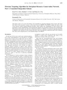
PUA_CNN

Fig.2. The initial topology of CNN based PUA

PUA_MFNN

During the first step of recruitment, each candidate neuron is connected to each of the input neurons, but not to the output neurons. The weights on connecting the input neurons and candidate neurons are adjusted to maximize the correlation between the output of each candidate neurons and the residual error at the output neuron, see Fig. 3. The pseudo connection shown in Fig. 3 is applied to deliver the error information from the output neurons but not to forward-propagate the output of candidate neurons. A number of passes over the training data are executed and the inputs of all the candidate neurons are adjusted after each pass.

Fig.1. The topology of MFNN based PUA ([12])

In this article, a modified PUA is implemented where the input and output elements remain the same; see Fig. 2. However, in this case the topology of the MFNN is then replaced by a CNN. The CNN architecture starts with a minimal topology, consisting only of the input and output neurons. The optimal values of the direct input-output synaptic weight links are computed during the training procedure using GPS derived position as updates). The training procedures continue with minimal topology for the entire training data set until no further improvement can be achieved. During this process, there is no need to back propagate the output position error (between the network output and the GPS updates) through hidden neurons. Any conventional training algorithm for single layer network (e.g. the standard gradient descent algorithm) can be applied. In this article, the Quickprop algorithm developed in [22] is implemented due to its simplicity and faster convergence speed [17]. To recruit a new hidden neuron, pools of candidate neurons that have different sets of random initial weights are applied. All the candidate neurons receive the trainable input connections from the external inputs and from all pre-existing hidden neurons. In addition, all candidate neurons receive the same residual error for each training pattern feedback from the output neurons as shown in Fig. 2. Thus, the recruitment of the first hidden neuron can be completed in a two-step process.

δ N PUA (t ) δ EPUA (t )

Output neurons

Step.2 A pool of candidate Hidden neurons (1st hidden layer) …

Input neurons

…

Fixed weights Weights under training (correlation maximization)

VINS (t ) φINS (t ) PUA_CNN

pseudo connection

Fig.3. Adding first hidden neuron (Step.2)

The goal of this adjustment is to maximize, S, the sum over all output neuron (o) of the magnitude of the correlation between (V), the output of a candidate neuron, and (Eo), the residual output error observed at unit (o), as

237

indicated in the following equation:

S = ∑ ∑ (V p − V )( E p ,o − Eo ) , o

Fig. 5. All the connections to the output neurons are then established and trained. Similar to Fig. 1, all the hidden neurons can be regarded as additional input neurons during the training of single layer of weights (Fig. 6).

(1)

p

The process of recruiting new neurons, training their weights from the input neurons and previously recruited hidden neurons, then freezing the weights and then followed by training all connections to the output neurons, is continued until the error reaches the goal of training or the maximum number of epochs. According to [16], an epoch is defied as the presentation of the entire training set to the neural network (or hidden units) is reached. The finalized topology (CNN) shown in Fig. 7 becomes a modified feedforward neural network with (n) hidden neurons and (n) hidden layers. In other words, each hidden layer will consist of only one hidden neuron.

where o is the network output at which the error E p,o is measured and p is the training pattern. The quantities V and Eo are the values of V and Eo averaged over all patterns. For detailed descriptions of this procedure, see [22]. The Quickprop algorithm is applied to adjust the incoming weights to maximize S. The S indices of the entire candidate neurons in the pool are computed simultaneously and the candidate neuron with the highest value of S is recruited after all the (S) indices stop improving; see Fig. 4.

δ N PUA (t ) δ EPUA (t ) Output neurons

Input neurons

Step.3

δ N PUA (t ) δ EPUA (t )

(2nd hidden layer) …

Input neurons

Fixed weights

VINS (t ) φINS (t ) Weights under PUA_CNN

Candidate pool

Output neurons

1st hidden neurons recruited

Step.4

Fixed weights

VINS (t )

training (Quickporp)

…

Weights under

φINS (t ) training (correlation

PUA_CNN

maximization)

Ghost connection

Fig.4. The recruitment of the first hidden neuron (Step.3) Fig.5. Adding the second hidden neuron (Step.4)

During the process of recruitment, only a single layer of weights is trained. The incoming weights of the winner neurons are frozen and the winner becomes the hidden neuron and is inserted into the active network in the second step of recruitment when the training is completed. The new hidden neuron is then connected to the output neurons and the weights on connection become adjustable. All connections to the output neurons are trained. In other words, the weights connecting the input neurons and the output neurons are trained again using the Quickprop algorithm. On the other hand, the new weights connecting the hidden neurons and output neurons are trained for the first time. The second hidden neuron is then recruited using the same process, as shown in Figs. 5 and 6. This unit receives input signals from both input neurons and previous recruited hidden neuron. All weights connecting input neurons and candidate hidden neurons are adjusted to recruit the second hidden neuron. The values of the weights are then frozen as soon as the hidden neuron is added to the active network; see

δ N PUA (t ) δ EPUA (t ) Output neurons

Step.5

2nd hidden neurons recruited

Input neurons

Fixed weights

VINS (t ) φINS (t ) Weights under PUA_CNN

training (Quickporp)

Fig.6. The recruitment of the second hidden neuron (Step.5)

238

The usage of CNNs for developing an alternative INS/GPS integration scheme poses several advantages over MFNNs. First, the best topology can be decided automatically based on the complexity of the applications. There is no need to perform extensive empirical trials to determine the size and depth of the network (i.e., the number of the hidden neurons and hidden layers, respectively). Moreover, the learning speed of CNNs is faster. In the standard back-propagation algorithm, the hidden neurons perform a complex interaction between each other before they settle into useful role. On the contrary, each of the hidden neurons of CNNs sees a fixed problem and can decisively be used to solve that particular problem. In addition, there is no need to propagate residual error signal through each hidden neuron.

outputs ( δN GPS (t) , δE GPS (t) ) are provided by GPS during signal availability in either DGPS or SPP mode of operation. As long as the GPS signals are available, the learning process continues to reduce the estimation error in order to obtain optimal values of the network parameters. In this case, the desired outputs ( δN GPS (t) , δE GPS (t) ) are used as the system output. Most of the neural network applications apply off-line trained weights to provide prediction of the network output [16]. However, in case of INS/GPS integration for navigation applications, it is required to track direction changes and mimic the motion dynamics using the latest available INS and GPS data. In other words, the synaptic weights should be updated during the navigation process to adapt the network to the latest INS sensor errors and the latest dynamics condition whenever the GPS signal is available. To implement such criterion, [2] proposed a window-based weights updating strategy to utilize the synaptic weights obtained during the conventional off-line training procedure (or probably from similar previous navigation missions). This criterion utilizes the latest available navigation information provided by the GPS signal window to adapt the stored synaptic weights so that they can be applied to mimic the latest motion dynamic and INS sensor error. Moreover, [2] demonstrated the advantages of the proposed strategy in terms of the prediction accuracy during GPS signal blockages in real time mode.

δ N PUA (t ) δ EPUA (t ) Output neurons

Input neurons

VINS (t ) φINS (t )

Recruited n hidden neurons (n hidden layers)

PUA_CNN PUA_CNN System Fig.7. Finalized CNN-Based PUA

DGPS/SPP

IMU

In Fig. 7, since only a single layer of weights is trained (due to the fact that the recruited hidden neurons are treated as additional input neurons), the residual error signal can be delivered to all hidden neurons at the same time. In addition, CNNs are useful for incremental learning, in which new information is added to a previously trained network. They can reflect the variation of the model complexity by adjusting their weights and topology automatically with aiding information. In contrast, MFNNs can only alter the weights to track the variation of model complexity

Position Difference

PUA INS Mechanization

+ -

∑

Position Difference

Learning Azimuth

System Output

GPS Outage

Velocity

IV. SYSTEM IMPLEMENTATION

Fig.8. Step.5, the recruitment of 2nd hidden neuron

Fig. 8 illustrates the INS/GPS system configuration and learning strategy of the proposed CNN-based scheme. The system receives the outputs (velocity and azimuth) from the INS mechanization at epoch t ( VINS (t) and φINS (t) ) and generates the coordinate differences between two consecutive epochs ( δN PUA (t) , δE PUA (t) ). The desired (reference)

V. RESUTLS AND ANALYSIS To evaluate the performance of the proposed CNN scheme compared to an extended KF, a MEMS IMU/GPS integrated system developed by the Mobile Multi-Sensor Systems (MMSS) research group at the University of

239

Calgary is used. Three field tests were conducted on March, 2004 using a navigation grade IMU (Honeywell CIMU), the MMSS group MEMS IMU (Analog Devices Inc. sensors) and two NovAtel OEM 4 GPS receivers (for providing DGPS as a reference GPS solution). The GPS measurements are processed using the NovAtel Waypoint GrafNavTM software in SPP mode. For each test, the GPS navigation solution is fed into AINS (Aided Inertial Navigation System) toolbox [23], a software that has been developed by the MMSS group, to obtain INS/GPS SPP integrated solution for further analysis. The reference trajectory for each test was generated by the CIMU/DGPS integrated system solution. The IMU and GPS measurements obtained in the first and second field tests were applied to generate the stored navigation knowledge. The third field test trajectory was used as the test trajectory for the proposed scheme. The first field test composed of a large loop; see Fig. 9. The duration of this field test was 1200 seconds. The DGPS navigation solution was not able to provide continuous position and velocity update due to the influence of several GPS outages. The second field test (Fig. 10) consisted of a straight-line segment and a large loop. The duration of this field test was 1000 seconds. Similar to the first test, the DGPS navigation solution was not available all the time due to the influence of several actual GPS outages. x 10

ADI-Training Trajectory (2)

6

x 10 5.677

INS/DGPS DGPS

5.676 5.675

North(m)

5.674 5.673 5.672 5.671 5.67 5.669 5.668 5.667 7

7.02

7.04

7.06

7.08

7.1

7.12 5

East(m)

x 10

Fig.10. 2nd field test

The third field test (shown in Fig. 11) consisted of six straight-line segments and eight sharp turns. The duration of this field test was 1800 seconds. Again, the DGPS navigation solution had several gaps due to GPS signal outages.

ADI-Training Trajectory (1)

6

5.671

hidden neurons. The topology remained fixed while the new information was fed in real-time with the windowing technique during navigation. In other words, the hidden neurons recruited during off-line training were able to cope with the dynamic variations and INS sensors errors during the test trajectory.

5.67

ADI-Tested Trajectory

6

5.678

x 10

North(m)

5.669

5.676 5.668

5.674

North(m)

5.667

5.666 INS/DGPS DGPS 5.665

7.02

7.03

7.04

7.05

7.06

East (m)

7.07

7.08

7.09

5.672

INS/DGPS outage(1) outage(2) outage(3) outage(4) outage(5) outage(6) outage(7) outage(8)

5.67 5.668 5.666

5

x 10

5.664

Fig.9. 1st field test

5.662 7

The stored weights were acquired using the measurements obtained through the first two field tests in the traditional off-line training mode. Furthermore, the window based weights updating strategy was applied to update the navigation knowledge during the availability of the GPS signal. Such strategy guarantees that the weights can be updated continually during navigation as long as new information is available. It is worth mentioning that the final topology of the CNN after off-line training consisted of 41

7.01

7.02

7.03

7.04

7.05

7.06

7.07

East(m)

7.08

7.09

7.1 5

x 10

Fig.11. 3rd field test

In this third test, the vehicle was driven through a residential area, inside a short tunnel, under an overpass and then through a forest area. Thus, eight actual GPS signal outages that include the impact from intermittent signal reception (i.e. through the forest area or urban canyon) or no

240

signal reception (i.e. under an overpass or inside a tunnel) took place along this trajectory. These outages are also shown in Fig. 11.

scheme (50 hidden neuron). Each hidden layer of the CNN based scheme consists only of one hidden neuron, and thus, the final topology of the CNN scheme became deeper than that of the MFNN (i.e. has more hidden layers). Based on the results presented in Fig. 12, the CNN based scheme is able to reach the same training goal with less training time and simpler architecture when compared to the MFNN based scheme. In addition, the CNN scheme distinguishes itself from the MFNN since it can decide its topology “on the fly” based on the dynamic variations and the presented INS sensor errors. Figs. 13 and 14 show examples of how the positional errors accumulated for different MEMS IMU/GPS SPP integration schemes (KF, CNN, MFNN) during some of the used 8 GPS signal outages. Table II gives the performance summary during all of the GPS signal outage periods.

Then, the different schemes were implemented using the CNN and MFNN approaches. The inputs and outputs of the MFNN based scheme are exactly the same as that of the CNN based scheme. However, the MFNN number of hidden neurons and layers were decided empirically. The MFNN was designed to have a nonlinear hidden layer and linear output layer. On the other hand, the topology of the CNN based scheme was decided automatically and all the hidden neurons were nonlinear (e.g. hyperbolic tangent sigmoid). A segment of the second field test data (1200 seconds) was applied first to evaluate the learning performance of CNN and MFNN in terms of the required learning time (number of epochs). The initial weights of each scheme were given randomly and the pool size of the candidate hidden neurons was four. Fig. 12 illustrates the learning time required by both schemes, respectively.

East(1)

10

0

-2

SSE

10

Position Error(m)

PUA-CCN, CNN Training Goal=1e-006,HU=36

10

10

-4

0

SSE

10

10

10

50

100

2

0

0

-20

-10

-40 0

10

30

-20 0

40

300

20

200

0

100

20

40

0

-2

0 60 0 Time(second)

-4

50

10

0

0

-50

10

20

30

-100 0

30

KF PUA-CNN

20

40

60

10

20

30

North(4)

East(4) 1000

20

North(3)

20

-10 0

10

North(2)

East(2)

200 KF PUA-CNN

500

10

20

East(3)

150

182 Epochs/30.362s PUA-MFNN, Training Goal=1e-006,HU=50

Position Error(m)

10

10

-20 0

-6

North(1)

20

0

-6

0

0

100

200

300

400

0

431 Epochs/113.954s Fig.12. Learning speed comparison

50

-200 100 0 Time(second)

50

100

Fig.13. Positional errors during 1st ~ 4th GPS outages (PUA_CNN)

From Fig. 12, the CNN based scheme converged at least twice faster than the MFNN based scheme with the same training data set and training goal. The number of hidden neuron recruited was 36, which was less than the number of hidden neurons decided empirically for the MFNN based

From Figs. 13 and 14, the KF position error accumulates over time. There is no argument about such time error growing trend once KF operates in prediction mode without updates from GPS. On the other hand, the positional errors of both PUA methods (MFNN and CNN)

241

behave differently. In general, if taking into account the relationship between the vehicle dynamic variations and position error accumulation, one can easily discover the strong correlation between them. In other words, the error behavior of the proposed schemes is affected by vehicle maneuvers.

Figs. 13 and 14, the performance of MFNN and CNN based schemes in position domain was similar in general. However, the proposed CNN based scheme was able to construct the topology by itself based on the complexity of the application encountered.

As indicated in Table II, both MFNN and CNN schemes were able to reduce the positional error during most of the GPS signal outage periods. The overall improvement reaches 55% and 69%, respectively. Figs 13 and 14 depict that the KF was able to provide better positioning accuracy during the first 5 to 10 seconds of GPS signal outage period in some scenarios. In contrast, both MFNN and CNN schemes outperformed KF when the outage length extends to 20 seconds or longer in most of the scenarios.

TABLE II POSITIONING ERRORS DURING GPS SIGNAL BLOCKAGES (USING KF, PUA_CNN AND PUA_MFNN SCHEMES)

East(1)

North(1)

10

10

0

0

Blockage no. 1 2 3 4 5 6 7 8

KF (MEMS IMU/GPS SPP) Blockage MAX_ N MAX_ E Length(s) (m) (m) 30 6.34 25.48 60 246.85 25.83 30 53.48 14.26 120 511.57 1016.6 60 85.66 102.17 120 1406.6 597.60 120 1491.3 1698.1 60 39.15 247.66

RMSE Total (m) 13.76 110.54 22.23 490.80 57.08 559.43 878.02 106.08

Blockage no. 1 2 3 4 5 6 7 8

PUA_CNN (MEMS IMU/GPS SPP) Blockage MAX_ N MAX_ E Length(s) (m) (m) 30 8.8 7.2 60 11.23 12.64 30 20.07 12.56 120 35.07 66.35 60 68.58 15.66 120 44.48 67.64 120 34.62 35.97 60 24.19 29.03

RMSE Total (m) 11.37 16.91 23.68 35.04 53.43 89.95 49.92 20.63

Blockage no. 1 2 3 4 5 6 7 8

PUA_CNN (MEMS IMU/GPS SPP) Blockage MAX_ N MAX_ E Length(s) (m) (m) 30 3.60 18.04 60 9.80 69.94 30 9.8 63.10 120 32.49 67.46 60 22.55 135.27 120 75.62 47.31 120 19.80 46.47 60 31.97 13.78

RMSE Total (m) 18.40 42.01 49.27 41.89 107.36 44.45 19.95 15.85

-10 -10

Position Error(m)

-20 -30 0

10

20

-20 0

30

East(2) 300

20

200

0

100

20

40

Position Error(m)

East(3)

10

0

0

-50

20

30

-100 0 500

1000

0

0

-500

50 100 Time(second)

40

60

10

20

30

North(4)

East(4) 2000

-1000 0

20

North(3) 50

10

30

KF PUA-MFNN

0 60 0 Time(second)

20

-10 0

20

North(2)

40

-20 0

10

KF PUA-MFNN

-1000 0

st

50

VI. CONCLUSIONS

100

This article proposed an intelligent and constructive INS/GPS integration scheme for low-cost MEMS Inertial Measuring Units (IMUs) using a Constructive Neural Network (CNN). Compared to fixed topology networks, such as Multi-layer Feed-forward Neural Networks (MFNNs), CNNs provide more flexibility to develop an alternative scheme as it can decide the topology including the size and depth automatically based on the complexity of

th

Fig.14. Positional errors during 1 ~ 4 GPS outages (PUA_MFNN)

On the other hand, although MFNN and CNN schemes suffered from minor degradation in terms of the positional error in some scenarios due to the impact of dynamic variation, they were able to reduce the time error growing impact and provide relatively stable solutions. Comparing

242

the application at hand. In other words, the intensive empirical trials required for MFNNs to decide the optimal topology can be avoided. The results presented in this article demonstrated that the Kalman Filter (KF) was able to provide better positioning accuracy during the first 5 to 10 seconds of GPS signal outage periods in some scenarios when a low-cost MEMS IMU/GPS system was used. However, due to the limitations of bias instability and noisy measurements of MEMS IMUs, the corresponding KF positioning accuracy degraded rapidly with time. On the other hand, when the MFNN or CNN schemes are implemented, the KF results were improved by more than 55%. Although the performance of MFNN and CNN schemes in position domain was similar in general, the proposed CNN scheme was able to autonomously construct the topology by itself on the fly. In addition, the CNN scheme was able to achieve similar performance when the prediction task was applied with less hidden neurons. Finally, the INS/GPS integration applications require a more flexible approach to track the dynamic variation of the vehicle and the INS sensor error variations. This is especially true when a low-cost IMU is used. In neural networks terminology, such requirement can be fulfilled by continuous learning to adjust the weights and by proper topology variation if applicable. With this requirement, a selfgrowing or constructive network such as CNN might be able to provide certain advantage over fixed topology network such as MFNN.

[4] [5] [6]

[7] [8]

[9] [10]

[11] [12]

[13] [14]

ACKNOWLEDGMENTS

[15]

This study was supported in part by research fund from the National Science Council of Taiwan (NSC 95-2221-E006-001), the Natural Science and Engineering Research Council of Canada (NSERC) and the Canadian Geomatics for Informed Decisions (GEOIDE) Network Centers of Excellence (NCE). Dr. Eun-Hwan Shin is acknowledged as a co-author of the AINS toolbox used in the article for providing the INS mechanization and INS/GPS extended Kalman filter.

[16] [17] [18] [19] [20] [21]

REFERENCES [1]

[2]

[3]

El-Sheimy, N., Osman, A., Nassar, S. and Noureldin, A. (2004): A New Way to Integrate GPS and INS: Wavelet Multi Resolution Analysis. Invited Paper, Innovation Column, GPS World, V.4, N.10, pp. 42-49, October. Chiang, K.W., El-Sheimy, N., and Noureldin, A. (2004): A New WeightsUpdating Method for Neural Networks based INS/GPS Integration Architectures, Measurement Science and Technology, Vol. 15, No.10, pp. 2053-2061. Chiang, K.W. (2004): INS/GPS Integration Using Neural Networks for Land Vehicular Navigation Applications, PhD Thesis, Department of Geomatics Engineering, The University of Calgary, Calgary, Canada , UCGE Report No. 20209.

[22]

[23]

243

Brown R.G. and Hwang P.Y.C. (1992): Introduction to Random Signals and Applied Kalman Filtering; John Wiley and Sons, New York. Vanicek, P. and Omerbasic, M. (1999): Does A Navigation Algorithm Have to Use Kalman Filter?, Canadian Aeronautics and Space Journal, Vol. 45, No. 3,Septmber,1999. El-Sheimy, N. and Abdel-Hamid, W. (2004): An Adaptive NeuroFuzzy Model to Bridge GPS Outages in MEMS-INS/GPS Land Vehicle Navigation,. ION GNSS 2004, Long Beach, California, USA, September 21-24. [Gelb A.(1974): Applied Optimal Estimation; MIT Press, Cambridge, England. Mohamed, A. H. (1999): Optimizing the Estimation Procedure in INS/GPS Integration for Kinematic Application. PhD Thesis, Department of Geomatics Engineering, The University of Calgary, Calgary, Canada, UCGE Reports No. 20127. Frykman, P. (2003): Applied Particle Filters in Integrated Aircraft Navigation System, MSc Thesis, Department of Electrical Engineering, The University of LinkÄoping, Sweden. Ojeda, L. and Borenstein, J. (2002): FLEXnav: Fuzzy Logic Expert Rule-Based Position Estimation for Mobile Robots on Rugged Terrain, The 2002 IEEE International Conference on Robotics and Automation, Washington DC, USA, May 11 - 15, pp. 317-322. Shin, E. H. and El-Sheimy, N. (2004): An Unscented Kalman Filter for In-Motion Alignment of Low Cost IMUs. IEEE PLANS 2004, Monterey, California, USA. Chiang, K.W. and El-Sheimy, N. (2002): INS/GPS Integration Using Neural Networks for Land Vehicle Navigation Applications, Proceedings of the ION GPS 2002 Meeting, Portland, Oregon, USA, September 24-27. Chiang, K.W., Noureldin, A., and El-Sheimy, N.(2003): Multisensors Integration using Neuron Computing for Land Vehicle Navigation, GPS Solutions. Vol. 6, No. 3, pp. 209-218. Chiang, K.W.(2003): The Utilization of Single Point Positioning and a Multi-Layers Feed-forward Network for INS/GPS Integration, ION GPS 2003 Meeting, September 9-12, 2003 Oregon Convention Center, Portland, Oregon, USA (CD). Chiang, K.W. and El-Sheimy, N. (2004): Artificial Neural Networks in Direct Georeferencing, Photogrammetric Engineering and Remote Sensing, July, 2004 Haykin, S. (1999): Neural Networks: A Comprehensive Foundation, 2 nd Edition, Prentice-Hall, New Jersey. Bishop, C.M. (1995): Neural Networks for Pattern Recognition, Oxford University Press. Ham, F.M. and Kostanic, I. (2001): Principles of Neurocomputing for Science and Engineering. McGraw-Hill. Alpaydin, E. (1991): CAL: Neural Networks that Grow When they Learn and Shrink when they Forgot, TR 91-032, International Computer Science Institute, May. Mezard, M. and Nadal J.P. (1989): Learning in Feed-forward Layered Networks: The Tiling Algorithm, J. Phys. A: Math. Gen., Vol.22, pp2191-22203 Frean, M.(1990): The Upstart Algorithm: A Method for Constructive and Training Feed-forward Neural Networks, Neural Computation, Vol.2, pp. 198-209 Fahlman, S.E. and Lebiere, C. (1990): The Cascade Learning Architecture, in Neural Information Processing System 2, Editors Touretzky, D., Morgan. Kaufmann Publishers, Inc., Denver, Colorado, pp. 198-209 Shin, E. H. and El-Sheimy, N. (2004), “Aided Inertial Navigation System (AINS®) Toolbox for MatLab® Software”, INS/GPS integration software, Mobile Multi-Sensor Systems (MMSS) Research Group, the University of Calgary, Canada.