A Content-Based Image Retrieval System for Surface Defects

A Content-Based Image Retrieval System for Surface Defects Jukka Iivarinen, Jussi Pakkanen and Juhani Rauhamaa∗ Helsinki University of Technology Laboratory of Computer and Information Science P.O. Box 5400, FIN-02015 HUT, Finland [email protected], [email protected] ABB Oy Paper, Printing, Metals & Minerals P.O. Box 94, FIN-00381 Helsinki, Finland [email protected] ∗

Abstract. In this paper a prototype system is described for the management and content-based retrieval of defect images in huge image databases. This is a real problem in surface inspection applications, since modern inspection systems may produce up to thousands of defect images in a day. We are using a noncommercial, generic content-based image retrieval (CBIR) system called PicSOM that is modified to fit to the special requirements of our application. The system is tested with a database of surface defect images using different kinds of features. Results indicate that the system works with a high level of success. Keywords: self-organizing map, content-based image retrieval, surface inspection, surface defects, MPEG-7 descriptors

1

Introduction

The need for efficient and fast methods for content-based image retrieval (CBIR) has increased rapidly during the last decade in many fields of industry and research. For example, modern surface inspection systems produce huge amounts of image data that has to be stored, managed, browsed, searched, and retrieved efficiently. The CBIR systems seem to be ideal tools for management of these huge image databases. The basic idea in CBIR is to find similar images without first labeling or annotating the images [1–3]. Instead some relevant features are extracted from the images, e.g. color histograms, texture features and shape features. These features are then stored in a database and indexed to speed up the retrieval process. What this means is that the search criterion is the image content, not some prior information that has been extracted by a human. One of the first and maybe still the best-known CBIR system is QBIC (Query by Image Content) [4], but several other commercial and noncommercial CBIR systems have been introduced during the last decade [3, 5]. The problem with these kinds of ready-made CBIR systems is that they are designed to be generic. Thus applying them to a specific problem is not always feasible nor efficient. There usually exists some problem-specific knowledge that could be utilized in the CBIR process, but this knowledge cannot be embedded to a generic system. Also these generic CBIR systems are usually not efficient enough to be used in demanding, real applications, such as surface inspection. Surface inspection of web materials is a challenging problem that consists of several subproblems, e.g. image acquisition, defect detection, and defect classification. In this paper we are dealing with management and content-based retrieval of surface defect images that 1

are obtained from a real, online paper inspection system. We have designed and realized a prototype CBIR system that is based on a noncommercial, generic content-based image retrieval system called PicSOM [6, 7]. Different feature descriptors (e.g. MPEG-7 descriptors [8]) are tested with a test database that has preclassified surface defect images. Some earlier work on the CBIR and classification of these kinds of images can be found e.g. in references [9, 10].

2

Surface Inspection Problem

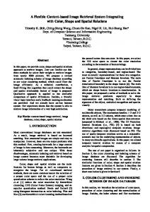
Paper mills utilize various methods to control the quality of their production. Laboratory tests are traditionally used for measuring precise values of different physical and chemical properties. In addition, on-line measurement systems are utilized for several quantities to enable real-time feedback control. Both of these methods are based on sampling, which is sufficient because paper properties are fairly continuous. However, there is a certain case of quality control that requires 100% coverage. That is web surface inspection. Its task is to find and report such anomalies that deteriorate the quality of final products or which are critical to the runnability and the condition of production equipment. Typical examples are different holes, spots, and wrinkles. Web inspection systems have been available for several decades. Their detection principle is normally based on optics. The sensors are applied to detect variations in the intensity of the light that is transmitting through or reflecting from the paper. Previously, on the basis of this information only the size and basic type of the defect were calculated. Because the detection was based on thresholding, the results did not tell very much about the causes of defects. However, reliable detection of basic defect types was as such very useful. The latest generations of web inspection systems utilize CCD linescan cameras as sensors. Due to high speed requirements, they first relied on various thresholding techniques. It was not until the end of the previous decade, when the advancements in digital electronics made it possible to convert the signal provided by CCD sensors to digital form in real-time [11]. As the result, modern inspection systems can now take electronic snapshots of surface defects in fast-moving paper webs with high accuracy. The main components of a web inspection system can be seen in Figure 1. The detection frame consists of a light source beam and a camera beam. The desired accuracy can be achieved by installing a suitable amount of cameras in the camera beam. A CCD line scan camera typically has a resolution of 1024, 2048 or 4096 pixels and the number of cameras in a systems is about 10 to 40. Since the paper web is moving, a two-dimensional image can be constructed by concatenating successive line images. The exposure time for a line is of the order of 100 microseconds or less. The resulting image resolution is typically about 1 mm in machine direction and a fraction of a millimeter in cross direction. The paper defect images with 256 shades of gray provide better insight about severity and origin of defects than before. Earlier, discrete defects were classified according to their main type of brightness (hole, light spot, or dark spot) and main dimensions or area. Now, the shape and internal structure of defects can be analyzed for more precise classification. For example, defects containing dark material can be caused by various substances present in paper process (fiber lumps, slime, coating splashes) or by external dirt (scale, oil), etc. However, due to the mechanisms of defect emergence, defect classification on the basis of appearance is not always obvious. The classes may be more or less fuzzy and overlapping, and thus exact labels cannot be given to them. Therefore, interpretation of defect images is a demanding task, even for an expert. Some example defect images are shown in Figure 2. A web inspection system may produce hundreds or even thousands of defect images in a day depending e.g. on the settings of the detection sensitivity. However, only the most severe defects require immediate action. The rest of the images can be saved in a history database for future analysis tasks. For management of such a huge database, suitable tools are needed. 2

Fig. 1. The main components of a web inspection system.

One of the key issues is to know which kind of defects are appearing in a specific papermaking process. Different papermaking processes in different paper mills produce different kind of defects, so the variability of defects is huge. It is not unusual that a web inspection system collects 50,000 defect images in a month. Most of these defects are of the common types. However, it is possible that the set contains samples of defects that occur very seldom or are completely new on that specific machine. Checking manually all these images is a tedious and time-consuming task. An automatic clustering tool, for example the self-organizing map (SOM), is necessarily needed. If the features describing the defects are selected properly, the occurrence of rare defect types can be indicated and used as a starting point for discovering the causes of these defects. A different case is the situation when a paper maker needs to know whether particular defect types are present in a database. A solution for this problem is described in the following chapters.

3

Content-Based Image Retrieval

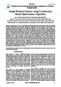
In content-based image retrieval, similar images are searched from a database based on the similarity of their visual features. These features may be simple, such as color histograms and distributions, or very complex, such as hierarchical descriptions of the items in the image. The similarity search can then be done using these feature vectors. The calculated features form a feature space. To proceed, we also need a way to measure distances between these feature vectors, in other words we need a metric for the data space. Usually the features consist of n real numbers, and the distances are measured with the Euclidean distance. When manipulating huge databases, a good index is a necessity. Processing every single item in a database when doing queries is extremely inefficient and slow. Raw image data is non-indexable as such, so the feature vectors must be used as the basis of the index. The problem we now face is that indexing data points in a multidimensional vector space is a nontrivial task. We propose to solve this image indexing problem by using the self-organizing map (SOM) [12] as an index to the images’ feature space data. The SOM is trained to match 3

Fig. 2. Some example defect images and their binary segmentation masks. The images are slightly scaled for visualization purposes.

the shape of the data in the feature space. After the training, the closest node in the SOM is calculated for every image in the database. This information about the closest nodes is stored. When a query is done, the first thing to be done is to calculate the closest SOM node, also know as the best matching unit (BMU), to the query image’s feature vector. When this is done, we know which images in the database are the closest to the query image: the ones that map to the same node as the query image. This cuts down processing time significantly. An added bonus is the hierarchy-preserving structure of the SOM. If we want to find more similar images, we can just examine the neighboring nodes of the BMU. 3.1

PicSOM Retrieval System

PicSOM has been developed in Laboratory of Computer and Information Science at Helsinki University of Technology to be a generic content-based image retrieval (CBIR) system for large, unannotated databases [6, 7]. It builds on the concepts of unsupervised clustering, self-organizing maps, and relevance feedback. The clustering property of PicSOM is very useful in our application since it makes it possible to automatically find relevant classes within defect images. This helps to detect the most severe defects or any other defect types of interest. PicSOM Training PicSOM works by first calculating a chosen number of feature sets for each image in the database. Several types of features can be used e.g. color, shape, texture, and structural features. Then a tree-structured self-organizing map (TS-SOM) [13] is trained with each feature set. TS-SOM is a basic building block of the PicSOM system. It is a treestructured vector-quantizer that has self-organizing maps (SOMs) at each of its hierarchical levels. The SOM sizes grow from top to bottom in a hierarchical way (see Figure 3). This kind of tree-structure makes training and searching much faster when compared to a normal, nonhierarchical SOM of the same size — the amount of computations is reduced from O(n) to approximately O(log(n)). After training each image is assigned to the closest map unit in each TS-SOM. Then the database can be searched. 4

Fig. 3. A diagram of the TS-SOM. The dashed lines show the links between parent and children nodes.

Relevance Feedback Every CBIR system needs some way of determining what the user wants to find. PicSOM uses the idea of relevance feedback to adapt to the user’s search criteria. First the user is shown a group of different kinds of images. The user then selects the ones that look like the image he is searching for. The system then looks what SOM nodes the images map to. Then it tries to find images that map to the same or neighboring nodes as the selected images and as far as possible from the discarded images. The best images are then shown to a user, who again selects the best ones and discards the rest. When this process is repeated the selected images should form clusters in the SOM grid. These can be seen in Figure 4 where the bottom levels of TS-SOMs are plotted. These so-called response maps show how important the particular TS-SOM is in the query. If the positive weights (red areas, marked with arrows) are spread then the map’s effect on the query is small, and if they are well clustered then the map’s effect is high. This way the system learns within few query iterations which maps (or feature sets) are important in each query.

4

Features for CBIR

Two types of features are of interest when considering defect images: shape features and internal structure features. Shape features are used to capture the essential shape information of defects in order to distinguish between differently shaped defects, e.g. spots and wrinkles. In addition to shape a defect has some kind of internal structure that consists of dark and light areas, holes, etc. Internal structure features are used to characterize the gray level and textural structure of defects. In this study we have experimented with our old features that we used in our defect classifier already in 1998 [9] and with the features of the MPEG-7 standard [14, 8]. The MPEG-7 standard ISO/IEC 15938, formally named “Multimedia Content Description Interface”, defines a comprehensive, standardized set of audiovisual description tools. It is not aimed at any one application in particular, instead it supports a broad range of descriptors for different types of multimedia information. The aim of the standard is to facilitate quality access to content, which implies efficient storage, identification, filtering, searching and retrieval of media. In addition to the still image descriptors demonstrated in this paper, the standard includes various descriptors for video and audio content. Furthermore, the standard enables the definition of new types of content descriptors. The existing MPEG-7 descriptors provide a framework for both high level semantic abstractions and low level abstractions such as shape, color and movement. For paper defect image retrieval, only the low level visual descriptors that can be extracted without human interaction are of interest. The feature 5

Fig. 4. The PicSOM user interface. At the top are the bottom levels of different TS-SOMs, then the previously selected images and finally the best results found. See text for further explanations

vectors corresponding to the MPEG-7 visual descriptors were extracted with the MPEG-7 eXperimentation Model (XM) software version 5.5. 4.1

Shape Features

There are a plenty of shape descriptors available [15, 16] that can be divided into two main categories: region-based and contour-based methods. Region-based methods use the whole area of an object for shape description, while contour-based methods use only the information present in the contour of an object. There are some techniques, for example, Fourier transforms and moments, that can be applied using both approaches with only small changes in algorithms. Using only contour information in shape analysis can be beneficial: – information inside the object’s contour is lost when dealing only with the contour (whether this is an advantage or a disadvantage, depends on the application) – it takes less space to store different objects (data compression) – shape descriptors are faster to calculate because there are less image pixels to process (although the overhead that comes from contour tracking must be included in total computation time) – variations in a contour are more easily detected 6

In case of surface defects the main interest is in the shape of a defect’s contour. A natural approach is thus to consider contour-based shape descriptors that can better capture the information that is present in contours. One such set of shape descriptors, simple shape descriptors (SSD), was proposed in [17] where it was noted that each of the proposed descriptors was insufficient for a complex recognition task, but a combination of them had good recognition capabilities and also low computation costs. The other two shape descriptors that are used in this study, the edge histogram (EH) and the region-based shape (RS), are from the MPEG-7 standard. Different kinds of edge histograms have been popular in various CBIR applications since they are powerful, fast to extract, and they do not require a segmentation mask (i.e., images do not need to be pre-segmented). The region-based shape is a standard region-based shape descriptor that (like the SSD) needs a segmentation mask. The shape descriptors utilized in this paper are: – Simple shape descriptors (SSD) calculate six features from defect’s border: convexity, principal axis ratio, compactness, circular variance, elliptic variance, and angle. They are translation, rotation (except angle), and scale invariant shape descriptors. – Edge histogram (EH) calculates the amount of vertical, horizontal, 45 degree, 135 degree and non-directional edges in 16 sub-images of the picture, resulting in a total of 80 histogram bins. – Region-based shape (RS) descriptor utilizes a set of 35 Angular Radial Transform (ART) coefficients that are calculated within a disk centered at the center of the image’s Y channel. In addition to the EH and the RS descriptors, the contour-based shape descriptor defined by MPEG-7 could also be of use. However, it produces vectors with varying amounts of components which requires a unique method for similarity matching. This makes it useless for our CBIR application. 4.2

Internal Structure Features

As already noted, we are using texture and gray level features to characterize defect’s internal structure. For texture description, we tested two methods: the co-occurrence matrix method (texture features (TEX)) and the homogeneous texture (HT) from the MPEG-7 standard. The co-occurrence matrix method, known also as the spatial gray-level dependence method, has been widely used in texture analysis since the early 1970’s [18]. It is based on repeated occurrences of different gray level configurations in a texture. It works well for a large variety of textures, especially for stochastic textures. The co-occurrence matrix is usually reduced to a set of features to decrease calculation time and memory requirements. The homogeneous texture implements another common technique called Gabor filtering. The texture features are: – Texture features (TEX) are calculated from the co-occurrence matrix. The co-occurrence matrix is formed to each defect and four texture features, energy, contrast, entropy, and mean, are calculated from it. – Homogeneous texture (HT) descriptor filters the image with a bank of orientation and scale tuned filters that are modeled using Gabor functions. The first and second moments of the energy in the frequency domain in the corresponding sub-bands are then used as the components of the texture descriptor. There is another texture descriptor in MPEG-7, called the texture browsing. However, XM 5.5 had problems calculating the texture browsing descriptor correctly. Because the homogeneous texture represents essentially the same qualities of an image (directionality, coarseness and regularity) but with more precision, the issues with the texture browsing were not further examined and the descriptor was omitted. 7

For gray level description, we tested the simple gray level histogram (GLH) and three descriptors from the MPEG-7 standard. The gray level (or color) features are: – Gray level histogram (GLH) is a 256-bin distribution of gray levels in a defect. – Color layout (CL) specifies a spatial distribution of colors. The image is divided into 8×8 blocks and the dominant colors are solved for each block in the YCbCr color system. Discrete Cosine Transform is applied to the dominant colors in each channel and the DCT coefficients are used as a descriptor. – Color structure (CS) slides a structuring element over the image. The numbers of positions where the element contains each particular color are stored and used as a descriptor. – Scalable color (SC) is a 256-bin color histogram in HSV color space, which is encoded by a Haar transform.

5 5.1

Experiments Image Databases

Our image databases have paper defect images that were obtained from a real, online paper inspection system. The images have different kinds of defects, e.g. dark and light spots, holes, and wrinkles. Their sizes vary according to the size of a defect. Some images are only 200 by 200 pixels in size while others are several thousand pixels high. All the images are in gray-scale with 256 gray levels. Some of the images are segmented after acquisition so that each image has a gray level image and a binary segmentation mask that indicates defect areas in the image. Segmentation of these kind of images is a very hard problem, and it cannot be done with simple gray-level thresholding techniques [19]. The image database with the defect segmentation masks were provided by ABB Oy. All further processing is done only for defect areas; we are thus omitting the noninteresting background (or normal, intact surface). It is important to get rid of the background since it usually covers most of the image. Thus it may spoil feature extraction and then the whole CBIR process; the point here is to find similar defects, not similar images. Especially the shape features need to have the segmentation information, otherwise they could not be extracted. On some occasions there was more than one defect in an image. In this case we only calculated the features of the largest defect. We have two different databases, a small one with labeled defects, and a large one with unlabeled defects. The first database has 1308 surface defect images. They are preclassified into 14 different classes with 100 images in 12 of the classes, 76 images in class number 11 and 32 images in class number 12. Example images from each class are depicted in Figure 5. The classes are based on the cause and type of a defect, and can therefore contain images that are visually dissimilar in many aspects. On the other hand, some classes are very hard to tell apart. This makes their classification with general-purpose visual descriptors an extremely challenging problem. Even a human cannot always differentiate between the images. For example, class 7, “oil spots”, contains many images that are practically impossible to distinguish from class 9, “clean holes”. The second database has approximately 45000 defect images. This database was used only in visual testing in Section 5.3 since the images were not preclassified. 5.2

KNN Classification

The performance of different descriptors with the smaller preclassified database was evaluated by performing a leave-one-out K-nearest neighbor (KNN) cross-validatory classification. Euclidean distance and K = 5 was chosen for all calculations. Some experiments were also 8

Fig. 5. Examples of the defect classes. Note how several of the classes are very similar, especially classes 11 and 12.

performed using L1-norm as the distance, but no significant difference in the performance was detected. We also tested some combinations of different feature sets. The combined results were obtained by retrieving the classes of the five nearest images for each feature set and determining the winning class by counting the total occurrences of each class. The KNN classifications were made primarily to select the best features that should be tested with the PicSOM CBIR system. Classification results are shown in Table 1. Clear winners can be found among the texture and the color features. These are the homogenenouos texture (HT) that really outperforms the TEX features, and the color structure (CS). The performances of the HT and the CS are really good, almost 80%. If we look at their results more closely, we see that the HT works significantly better than the CS with classes 3, 7, 9, and 10, but the CS is better with classes 2, 5, and 13. So none of them is better with all the classes. The shape descriptor results are not so clear. The edge histogram (EH) is the best one with the simple shape descriptors (SSD) following. But the SSD is much better than the EH with classes 2 and 8, and equally good with classes 4, 6, 9, 10, and 14. So the SSD seems to be quite useful for classification of these kinds of images. The region shape (RS) performed poorly. Finally there some combined classification rates in Table 1. When all the MPEG-7 feature sets were combined the classification rate of 85% was obtained. This is not an optimal approach since these feature sets have a lot of redundant information. When using a combination of the best three feature sets (HT, CS, and EH), the classification rate of 87% was obtained. This can be considered a really good result for our database. We also tested the performance of our old features (SSD, TEX, and GLH). Their combined classification rate was only 70% which is still quite acceptable but is far worse than with the best MPEG-7 feature sets. 9

Table 1. Classification results.

Shape features

EH SSD RS Texture HT features TEX Color CS features GLH SC CL EH,HT&CS All MPEG-7 SSD,TEX&GLH

Classification rates (%) 1 2 3 4 5 6 61 25 68 91 55 23 50 44 47 88 37 24 54 27 37 52 35 26 96 54 71 89 74 82 30 59 38 98 39 14 97 75 60 88 82 78 98 73 39 92 57 49 75 6 28 69 39 74 85 11 11 64 41 78 99 79 77 98 84 89 98 68 75 96 84 85 96 81 58 100 66 48

of different classes 7 8 9 10 11 76 37 64 69 79 41 77 65 72 14 43 34 45 57 38 97 65 91 94 75 69 41 48 19 5 70 59 77 62 76 1 89 26 42 13 90 17 6 18 70 23 32 14 33 63 98 74 95 96 81 97 77 95 94 71 64 92 68 78 13

12 11 4 0 0 7 15 0 0 4 11 11 0

13 78 30 35 64 53 86 40 46 31 91 90 60

14 avg 91 61 91 52 88 42 93 79 40 42 95 76 79 53 60 44 39 39 98 87 99 85 94 70

We also ran the same tests without the segmentation masks to see how the masks would affect the classification rates. The shape features (SSD and RS) were not tested since their calculation needs these masks. The results were quite surprising. For example, when using the combination of the best three MPEG-7 feature sets (HT, CS, and EH), the classification rate dropped from 87% to 80%. When all the five MPEG-7 descriptors (excluding RS) were combined, the classification rate dropped only 3%. So it is possible to use these features successfully even without the segmentation masks. Class 12 is recognized miserably with each descriptor because of several reasons: the size of the class is smaller than the others, images are very similar with each other, and many images also look a lot like the images in classes 3 and 5. The outcome of all this is that the performance is sometimes worse than random guessing. 5.3

CBIR Experiments

PicSOM has a built-in method of evaluating the retrieval results, which mimics the way a human does searching on the system. You tell it which defect class you want to test and which features to use. It then seeks a single example image belonging to that class to start the query. Then it seeks the best matches to the query and selects all returned images that belong to the desired class. All these selected images are then used as a search criterion for another search. Again the found correct images are added to the query criterion and a new query is performed. This process continues until a prespecified number of iterations is reached. The results are data vectors, containing the recall and precision values for each iteration. Recall means the percentage of correct images retrieved so far. When recall reaches 100%, all desired images have been found. Precision tells how many of all returned images belong to the correct class. A minimum requirement of any CBIR system is that precision should be higher than the a priori probability of the queried class. Otherwise the system is worse than just selecting images in the database at random. The tests were run separately for every class. The test results were then loaded into Matlab for analysis. We ran tests both using a single feature and a combination of several features in the query. Results with the small database First we tested how the PicSOM results compare to the KNN results from the previous section. Due to the nature of the PicSOM system, we 10

Fig. 6. Query results with PicSOM. In the first graph the three best MPEG-7 descriptors (HT, CS, and EH) are used. The second has these features, and also the additional shape feature (SSD).

cannot easily get exact classification percentages. We need some kind of a measure that is comparable to those. It is reasonable to assume that a human would do at most ten iterations of searching before quitting. Therefore we ran PicSOM’s tester and examined the recall rates after five and ten iterations. These values are not exact classification rates, but they describe quite well the system’s performance. The more images of the correct class the system returns the better the recall value. A value of 100% means the query target has been fulfilled optimally, since all images of the desired class have been found. It should be noted that in the optimal case recall could be 100% after five queries. This requires that the system works perfectly, so in practice this is never reached. The results of these tests can be seen in Figure 6. The first thing to notice is that doing ten iterations instead of five noticeably increases the recall rate. The increase is approximately 20–30% in almost every case. This is a good result, as it shows that PicSOM can improve its search results by doing a bit of extra work. The percentages are very much like the ones obtained with KNN. The recall rates are approximately 55% after five iterations and 80% after ten iterations. These results can be considered quite good, given the data set’s difficult nature. It should be noted that the classes that are easy for the KNN classifier are also easy for PicSOM. However PicSOM seems to do slightly better on the very difficult classes 11 and 12. This can not be proved conclusively, though, given the different nature of the recall values and classification percentages. When we compare the two graphs in Figure 6, we find that adding the problem specific shape features improves the query results. The average increase is approximately 6%, from 77% to 83%. This is a very noticeable improvement and also proves that PicSOM can effectively combine different features to obtain a better query result. Another way to characterize the system is using precision/recall graphs. Examples of these can be seen in Figure 7. Each one contains two graphs, one for an easy class and one for a difficult class. The upper graph has the three best features color structure, homogeneous texture, and edge histogram. The lower one has these and the shape feature set (SSD). These graphs show again how PicSOM can combine different feature sets effectively. When using all four feature sets, precision is clearly higher on the easy class when the recall values start to approach one. The difficult class has also noticeably higher precision throughout. It should 11

Three best features 0.9 Easy class Difficult class 0.8

0.7

Precision

0.6

0.5

0.4

0.3

0.2

0.1

0

0

0.1

0.2

0.3

0.4

0.5 Recall

0.6

0.7

0.8

0.9

1

Three best features and shape 0.9 Easy class Difficult class 0.8

0.7

Precision

0.6

0.5

0.4

0.3

0.2

0.1

0

0

0.1

0.2

0.3

0.4

0.5 Recall

0.6

0.7

0.8

0.9

1

Fig. 7. Two precision/recall graphs characterizing the system.

be noted that these performance boosts happen also at the most difficult cases, which is a very desirable feature. Another thing the graphs in Figure 7 have in common is that their precision increases after the first couple of iterations. This is a very desired feature of the PicSOM system. This increase indicates that PicSOM is able to learn what kind of images the user was searching. It should be noted that this learning is done based only on the feedback information gathered during the queries. This characteristic was noted in almost all of the tests we performed. Another way to look at the recall values can be seen in Figure 8. It shows the amount of found images as the number of iterations increases with two different feature sets. The curves rise very steeply at the beginning, meaning that the query results are very good. The system only starts to slow down after 80%–90% of the desired images have been found. This happens after approximately 10 iterations, which is consistent with the results of Figure 6. The results regarding feature selection differ slightly from the KNN results where we obtained 2% better results with the three best MPEG-7 features than with all of the MPEG-7 features. In PicSOM the three best MPEG-7 features, color structure, edge histogram and homogeneous texture, yielded slightly worse results than all of the features. This can be seen in Figure 8 where the graphs on the upper figure are not as steep and go slightly lower than the graphs on the lower figure. This is due to PicSOM’s ability to efficiently combine different feature sets and to automatically give more value to those feature sets that are 12

1

0.9

0.8

0.7

Recall

0.6 Easy class Difficult class Average

0.5

0.4

0.3

0.2

0.1

0

0

5

10

15

20

25 Iterations

30

35

40

45

50

45

50

1

0.9

0.8

Easy class Difficult class Average

0.7

Recall

0.6

0.5

0.4

0.3

0.2

0.1

0

0

5

10

15

20

25 Iterations

30

35

40

Fig. 8. Recall values as a function of the number of query iterations. The upper one uses all MPEG-7 features, the lower one has the three best ones.

important in a current query. So one could say that in most cases PicSOM benefits from new feature sets. Some example query results are shown in Figure 9. The leftmost image in each row was used as an initial query image. The four rightmost images are the best matches after 3-4 queries. At each query PicSOM returned 5 images of which the best ones were selected. This way we were trying to imitate the actual use of the PicSOM system where the user gives one image and tries to find within few queries similar images from the database. Results with the large database Content-based image retrieval is usually applied to very large image databases that have thousands or tens of thousands of images. To test the suitability and scalability of our system to this task, we have tested it with another database that has 45 000 images. This testing has its own set of problems. As was noted earlier, preclassifying the image data is a very hard task that requires an expert. The amount of time and money required to preclassify an image database of this size is beyond our reach. Therefore these tests are run on a non-classified database. This means that the results are qualitative and fuzzy rather than exact, measurable and repeatable numbers. The system scales very well. The queries are completed almost in real time, even though the database size is ten-fold. The query results also seem very sensible when examined by visual inspection. The query results are very similar to the desired images and the system 13

Fig. 9. Some example query results.

adapts if the query target is modified during the search. These results suggest that the system retains a high level of success when used with large databases. However, it should be noted that we can not prove this conclusively, due to the lack of a proper, classified database.

6

Conclusions

In this paper we have proposed and evaluated a content-based image retrieval system for surface defect images that is based on PicSOM. The task of this system is to find similar images in a large, unannotated image database. For each image a set of visual descriptors is calculated and a TS-SOM is trained for each feature set. Using these and relevance feedback obtained from the user, images of the desired type can be found fast and efficiently. The PicSOM system is very efficient in combining different feature sets. This can be easily seen e.g. in Figure 7. Adding a shape feature set makes the precision levels go higher in the difficult stages of the queries. The decrease in precision when recall approaches 100% is not as strong when using more features. Not only can PicSOM efficiently combine different feature sets, but it can also automatically give more value to those feature sets that are important in a current query. Another result of our research is showing that the MPEG-7 color and texture descriptors can be used as features in machine vision problems. Their performance on these rather difficult surface defect images is surprisingly good. Of course, these tests do not guarantee the usability of MPEG-7 descriptors in the general case. It does, however, imply that MPEG-7 descriptors are worth experimenting with. 14

Acknowledgments The authors wish to thank Mr A. Ilvesmäki for the work with the MPEG-7 descriptors and the KNN classifications, and the PicSOM group (J. Laaksonen, M. Koskela, S. Laakso, E. Oja) at Helsinki University of Technology. The financial support of the Technology Development Centre of Finland (TEKES’s grant 40120/03) is gratefully acknowledged.

References 1. Y. Rui, T. S. Huang, and S.-F. Chang, “Image retrieval: Current techniques, promising directions, and open issues,” Journal of Visual Communication and Image Representation 10(1), pp. 39–62, 1999. 2. A. Del Bimbo, Visual Information Retrieval, Morgan Kaufmann Publishers, Inc., 1999. 3. O. Marques and B. Furht, Content-Based Image and Video Retrieval, Kluwer, 2002. 4. M. Flickner, H. Sawhney, W. Niblack, J. Ashley, Q. Huang, B. Dom, M. Gorkani, J. Hafner, D. Lee, D. Petkovic, D. Steele, and P. Yanker, “Query by image and video content: The qbic system,” IEEE Computer 28, pp. 23–32, Sept. 1995. 5. B. Johansson, “A survey on: Contents based search in image databases,” tech. rep., Linköping University, Department of Electrical Engineering, http://www.isy.liu.se/cvl/Projects/VISITbjojo/, Dec. 2000. 6. J. Laaksonen, M. Koskela, S. Laakso, and E. Oja, “PicSOM - content-based image retrieval with self-organizing maps,” Pattern Recognition Letters 21(13-14), pp. 1199–1207, 2000. 7. J. Laaksonen, M. Koskela, S. Laakso, and E. Oja, “Self-organising maps as a relevance feedback technique in content-based image retrieval,” Pattern Analysis and Applications 4(2+3), pp. 140– 152, 2001. 8. B. S. Manjunath, P. Salembier, and T. Sikora, eds., Introduction to MPEG-7: Multimedia Content Description Interface, John Wiley & Sons Ltd., 2002. 9. J. Iivarinen and A. Visa, “An adaptive texture and shape based defect classification,” in Proceedings of the 14th International Conference on Pattern Recognition, I, pp. 117–122, (Brisbane, Australia), Aug. 16–20 1998. 10. J. Iivarinen and J. Pakkanen, “Content-based retrieval of defect images,” in Proceedings of Advanced Concepts for Intelligent Vision Systems, pp. 62–67, (Ghent, Belgium), Sept. 9–11 2002. 11. J. Rauhamaa, T. Järvenpää, J. Moisio, and S. Taniguchi, “Paper web inspection with imaging capabilities,” in Proceedings of the 2000 Japan TAPPI Annual Meeting and Pan Pacific Conference, Special Lecture 2, Technical Sessions, pp. 369–379, (Sendai, Japan), Oct. 18–20 2000. 12. T. Kohonen, Self-Organizing Maps, Springer, Berlin, 3. extended ed., 2001. 13. P. Koikkalainen and E. Oja, “Self-organizing hierarchical feature maps,” in Proceedings of 1990 International Joint Conference on Neural Networks, II, pp. 279–284, (San Diego, CA), 1990. 14. B. S. Manjunath, J.-R. Ohm, V. V. Vasudevan, and A. Yamada, “Color and texture descriptors,” IEEE Transactions on Circuits and Systems for Video Technology 11, pp. 703–715, June 2001. 15. S. Marshall, “Review of shape coding techniques,” Image and Vision Computing 7, pp. 281–294, Nov. 1989. 16. M. Sonka, V. Hlavac, and R. Boyle, Image Processing, Analysis and Machine Vision, Chapman & Hall Computing, London, 1993. 17. J. Iivarinen, M. Peura, J. Särelä, and A. Visa, “Comparison of combined shape descriptors for irregular objects,” in Proceedings of the 8th British Machine Vision Conference, 2, pp. 430–439, (University of Essex, UK), Sept. 8–11 1997. 18. R. Haralick, K. Shanmugam, and I. Dinstein, “Textural features for image classification,” IEEE Transactions on Systems, Man, and Cybernetics SMC-3, pp. 610–621, Nov. 1973. 19. J. Iivarinen, K. Heikkinen, J. Rauhamaa, P. Vuorimaa, and A. Visa, “A defect detection scheme for web surface inspection,” International Journal of Pattern Recognition and Artificial Intelligence 14, pp. 735–755, Sept. 2000.

15