A CONTROL ARCHITECTURE FOR MULTIPLE SUBMARINES IN COORDINATED SEARCH MISSIONS Jo˜ao Borges de Sousa ∗,1 Karl Henrik Johansson ∗∗,2 Alberto Speranzon ∗∗,2 Jorge Silva ∗∗∗,1
∗
Dept. de Engenharia Electrot´ecnica e Computadores Faculdade de Engenharia da Universidade do Porto Rua Dr. Roberto Frias, 4200-465, Porto, Portugal E-mail:
[email protected] ∗∗ Dept. of Signals, Sensors & Systems Royal Institute of Technology, SE-100 44 Stockholm, Sweden E-mail: {kallej,albspe}@s3.kth.se ∗∗∗ Instituto Superior de Engenharia do Porto, Rua Dr. Ant´onio Bernardino de Almeida, 431, 4200-072 Porto, Portugal
Abstract: A control architecture for executing multi-vehicle search algorithms is presented. The proposed hierarchical structure consists of three control layers, which consist of maneuver controllers, vehicle supervisors, and team controllers. The system model is described as a dynamic network of hybrid automata in the programming language Shift and allows us to argue about specification, verification and dynamical properties in a formal setting. The particular search problem that is studied is that of finding the minimum of a scalar field using a team of autonomous underwater vehicles. As an illustration, a coordination scheme based on the Nelder-Mead simplex optimization algorithm is presented and illustrated through simulations. Keywords: Hierarchical controllers, autonomous vehicles, hybrid systems, search methods, simulation languages, supervision.
1. INTRODUCTION The problem of coordinating the operations of multiple autonomous underwater vehicles (AUV’s) in the search for extremal points in oceanographic scalar fields is addressed in the paper. The coordination entails exchanging real-time information and commands 1
This research has been partly supported by Agˆencia de Inovac¸a˜ o under project PISCIS. The PISCIS (Multiple Autonomous Underwater Vehicles for Coastal and Environmental Field Studies) project concerns the design and implementation of a modular, advanced and low-cost system for oceanographic data collection. 2 K. H. Johansson and A. Speranzon are partially supported by the European Commission through the RECSYS and the RUNES projects and the Swedish Research Council.
among vehicles and controllers whose roles, relative positions, and dependencies change during operations. There are several aspects to this problem: the organization of valid configurations of vehicles and controllers; the structure of each specific configuration; and the reconfiguration of these structures. Our approach to the problem is to structure the system into a control hierarchy, which consists of maneuver controllers, vehicle supervisors, and team controllers. The maneuver controllers implement elemental feedback control maneuvers for the AUV’s. Each AUV has attached a vehicle supervisor, which makes decisions on what maneuver to execute. The team controllers run the multi-vehicle coordination algorithm, but also
this state the vehicles in V exchange measurements to evaluate g and to determine spatial–temporal rendezvous points. In the motion state the vehicles then move to their designated rendezvous points. When they reach these points, a transition to the coord takes place and a new step begins. In the motion state it may happen that the transition to coord is not taken due to a communication time-out. In this case a transition to backtrack is taken. In backtrack the vehicles move to their previous locations at the end of the previous coord state and attempt to re-start the algorithm. If this is not possible, then a transition to ind is taken. In ind each vehicle executes its version of the algorithm independently, without coordinating with the other vehicles. Fig. 1. System specification handles structural adaptation and reconfiguration for the system of AUV’s. The controllers and their interactions are described as interacting hybrid automata using Shift, which is a programming language for dynamic networks of hybrid automata (Deshpande et al., 1997). The paper is organized as follows. In section 2 we introduce the problem formulation and the system specification. In section 3 we describe the input–output behavior of the components and how they interact as a dynamic network of hybrid automata. In section 4 we describe the controllers and how they organize the system and implement the reconfiguration strategies. Section 5 describes some guaranteed team behavior. The implementation of an optimization-based multivehicle search strategy is presented in section 6 together with some simulation results. In the appendix we present an aside on the Shift programming language.
2. PROBLEM FORMULATION We consider a class of search algorithms for multivehicle systems that are characterized by (1) one, or more, initial points in R3 ; (2) a measurement function m : R3 → R from locations in the 3-dimensional space to measurements of a given scalar field; (3) a sequence L of visited locations and measurements; (4) a way-point generation function g : L → R3 , which returns the next point to visit; and (5) a termination criteria. The multi-vehicle system has constrained communication range and highly nonlinear dynamics. Environmental constraints are given as bounded disturbances in the equations of motion. Let us describe the system specification S. Given a set of n vehicles V = {v1 , . . . , vn }, we define the system Σ as being V together with the controllers. The specification S for Σ that we consider in this paper is depicted in figure 1. It is given by a hybrid automaton that defines a class of search algorithms, and is further described in the sequel. Execution proceeds in steps as the search algorithm. The initial state is coord. In
Problem 1. Given a multi-vehicle system Σ and a specification, derive the controllers, configurations, and the reconfiguration strategies for Σ to execute the specification with guaranteed properties, such as continuation, termination, bounded-time execution, robustness with respect to model disturbances and communication constraints, and graceful degradation. Here we take a variation of this problem. We introduce a set of controllers, configurations and reconfiguration strategies and prove that it implements the specification with guaranteed properties.
3. COMPONENTS AND INTERACTIONS 3.1 Execution concepts We use the concept of maneuver, a prototype of an action description for a single vehicle, as the atomic component of the execution control. Thus we abstract each vehicle as a provider of maneuvers, which allows for modular design and verification. The maneuvers required to execute the search algorithm are only the following goto and hold commands: • goto(x, y, z, R, T ): reach the ball of radius R centered at (x, y, z) within time T ; • hold(D): execute a holding pattern for time D. We will prove that the implementation of the specification is as follows. At each step, there is a coordination stage and a motion stage. In the coordination stage the AUVs in V execute a hold maneuver and communicate to evaluate the way-point generation function g and to generate spatial-temporal rendezvous points for each of them. In the motion stage the vehicles execute goto maneuvers to reach their designated rendezvous points where a new coordination stage takes place. We have structured our design in a 3-level control hierarchy. Proceeding bottom-up there are the maneuver controllers (one per type of maneuver), vehicle supervisors (one per AUV), and the team controllers (one per AUV). We describe it next. First, we describe
We access the output variable s of v1 with the Shift construct s(v1). Here, we have used the link to v1 to read the output variable s. Shift allows the user to change link variables. We use this feature to create and maintain dynamic networks of hybrid automata. For example, we can change the value of the link variable t of v1 with the following construct t(v1):= tc2. In this example this construct is used to change the team controller of v1. This way we are are to change the input/output relations among components. 3.3 Controllers Fig. 2. Control hierarchies and links the AUV model. Second, we describe the data models for these controllers, which are modelled as hybrid automata. Third, we describe the legal configurations of input/output relations for the system.
3.3.1. Maneuver controller We use the objectorientation of Shift to define a hierarchy of maneuver controllers. At its root there is the elemental maneuver type MController. The other maneuver controllers inherit from this one. Its Shift data model is type MController { input array(number) ss; number x,y,z; mspec m;
3.2 AUV model We have adopted the notation from the Society of Naval Architects and Marine Engineers (SNAME) (Lewis, 1989) for the equations of motion. It is convenient to consider two coordinate frames: body-fixed and earth-fixed. The motions in the body-fixed frame are described by 6 velocity components η respectively, surge, sway, heave, roll, pitch, and yaw, relative to a constant velocity coordinate frame moving with the ocean current. The components of position and attitude in the earth-fixed frame are ν = (ν1 , ν2 ) = [x, y, z, φ, θ, ψ].
// state of all components // motion state // maneuver specification
output array(number) u;// control settings for actuators ... }
There may be several implementations for the same type of maneuver. Again, we use inheritance to specify the implementations of a maneuver type. 3.3.2. Vehicle supervisor the vehicle supervisor is
The Shift data model for
type supervisor { input /* what we feed to it */ TeamController tc;// link to team controller state /* whats internal */ MController mc; // link to maneuver controller mspec mt;// current maneuver specification array(number) ss;// state of all components ...
η˙ = f (t, η, ν, u, v), u(t) ∈ P (t), v(t) ∈ Q(t), (1) where u is the control and v the disturbance, and P (t) and Q(t) are closed sets in Rm . We consider the standard conditions for uniqueness and prolongability of the solutions for t ≥ t0 .
discrete /* discrete modes of behavior */ Exec, Error, Idle; // 3 discrete states transition Idle -> Exec {} ... ...
The Shift type definition for the AUV model is } type AUV { input /* what we feed to it */ array(number) u; // control settings array(number) v; // disturbances output /* what we see on the outside */ supervisor s; // link to supervisor TeamController t; // link to team controller number x,y,z; // motion state array(number) ss; // state of all components ... }
An instance of a type is called a component. We create an instance of a type with a create statement. In the following example we create an instance v1 of the AUV type with the output link variables s and t bound to components sup1 and tc1 respectively. Link variables refer to other components. v1 := create(AUV, s:=sup1, t:=tc1);
It interacts with tc through the exchange of the following input/output typed events: In command(m) – execute maneuver specification m. In abort – abort current maneuver. Out donev – completion of current maneuver. Out errorv(ecode) – error of type ecode. The typed events exchanged with mc are: Out exec(m) – launch maneuver controller to execute maneuver specification m. In donev – maneuver reached completion. In errorm(code) – error of type code. The transition system for this hybrid automaton is briefly described next. In the Idle state, the supervi-
sor accepts a maneuver command, In command(m), from the team controller tc, and takes the transition to Exec. On this transition it creates a MController named c of type specified in m and sets the state variable mc to c. The transition from Exec to Idle is taken when an abort command is received from tc, or when a In donev event is received from c. On this transition the state variable mc is set to nil. 3.3.3. Team controller Each AUV component has a TeamController. The Shift skeleton is type TeamController { input set(AUV) V; supervisor s; state number number number number
step; x,y,z; T1, T2, T3; c;
// AUVs in the team // link to its supervisor
// // // // // array(array(number)) L;// number t; //
last step (x, y, z) at last step coordination times counts measurements received visited locations timer
output TeamController m;// link to master TeamController set(TeamController) tc;// links to TeamController symbol role; // $master or $slave symbol nstate; // name of discrete state // $Init, $Error, $TMaster, // $TSlave, $SingleN, $SingleI mspec ms; // maneuver under execution set(array(number)) specs; // target regions discrete /* discrete modes of behavior */ Init, Error, TMaster, TSlave, SingleN, SingleI; ... }
It interacts with tc through the exchange of the following input/output typed events: Out command(m, T 1, T 2, T 3) – execute a maneuver specification m with coordination times [T1, T2, T3] In measurement(m) – measurement m. There are 6 discrete states. The last four, TMaster, TSlave, SingleN, SingleI concern the execution of the search algorithm. In the TMaster state it receives measurements from all vehicles in V, calculates the next way-point, and sends out the goto maneuver specifications to the other vehicles through the link tc. In TSlave it sends measurements to the master m and waits for goto maneuver specifications from ms. In SingleN it executes the goto maneuver specification received from the master and, upon its completion, it executes a hold maneuver. In SingleI it executes a goto maneuver to the position x,y,z at the last step. For each specific implementation we create several instances of the controller and AUV types. For example, v1:= create(AUV, s:=sup1, t:=tc1); v2:= create(AUV, s:=sup2, t:=tc2); V := {v1, v2};
The master and slave roles of TeamController can be changed during execution. In this implementation one TeamController is initialized to master and the others to slave and these roles do
not change. For example, the following construct m:=self is used in the initialization of the master TeamController.
3.4 Configurations Links among components of type TeamController change while the system implements the specification: in the motion state the vehicles are not required to communicate and these links may be nonexistent or nil; in the coord state the vehicles are required to communicate and these links have to be re-established. We use the term configuration to denote a set of components and links. This provides for a compact notation to describe execution properties. We need four configurations to execute the specification: ccoord; cmotion; cbacktrack; and cind. These configurations concern only team controller components, which are represented by the dashed arrow in figure 2. The ccoord configuration is described next ∃1 v ∈ V, ∀v ∈ V \v : m(tc(v)) = m(tc(v)) (2) ∧m(tc(v)) = tc(v) ∧tc(tc(v)) = {tc(v1 ), . . . , tc(vn )} ∧step(tc(v)) = step(tc(v)) ∧nstate(tc(v)) = $T master ∧nstate(tc(v)) = $T Slave In ccoord there is a master team controller which resides in v (it is the master of itself). In this controller the value of nstate is Tmaster; in the other controllers its value is TSlave. The link variable m is set to the master. The master is linked to the other controllers. The controllers are in the same step of the master: step(tc(v)) = step(tc(v)). The vehicles in V have to satisfy the communication constraints for those links to exist. In the cmotion configuration some of the links from the ccoord configuration may not have been removed. ∃1 v ∈ V, ∀v ∈ V \v : m(tc(v)) = m(tc(v)) (3) ∧m(tc(v)) = tc(v) ∧step(tc(v)) = step(tc(v)) ∧nstate(tc(v)) = $T master ∧nstate(tc(v)) = $T Slave The cbacktrack and cind configurations are defined respectively as
∃1 v ∈ V, ∀v ∈ V \v : m(tc(v)) = tc(v)
(4)
∧step(tc(v)) = step(tc(v)) nstate(tc(v)) = $SingleN ∧nstate(tc(v)) = $SingleN and ∀v ∈ V : m(tc(v)) = tc(v) ∧
(5)
nstate(tc(v)) = $SingleI We remark that configuration is a global concept. We do not manipulate configurations directly in our controllers. However, the controllers ensure that the system alternates between the coordination and the motion configurations while executing the specification (in the absence of faults). We describe how in the following section.
Fig. 3. Master mode operation
4. EXECUTION CONTROL Execution control commands vehicles and organizes controllers to execute the specification in a distributed fashion. The system implementation of a subset of the specification automaton (normal execution when the states alternate between coord and move) is described next.
4.1 Team controller In this implementation the initial allocation of the master and slave roles does not change. Hence, and for the sake of simplicity, two independent transition systems for each of the discrete states TMaster, TSlave are described separately. Consider those as two distinct automata. Consider TMaster and refer to figure 3 (the transitions are labelled with guards and actions; the guards are written in boldface; the arrows indicate the origins or destinations of the events). When the system enters a new step the counter c is set to zero and the coordination times T1, T2, T3 set to define the time window for coordination. The master AUV is required to reach its way-point during [T1, T2]. During [T2, T3] it receives measurements from the other vehicles and updates the counter c. When c=n it generates the new set of way-points for each vehicle, the coordination times for the next step, increments the step counter, sends the new coordination times T1, T2, T3 to the AUV’s and commands them to execute the corresponding goto maneuvers. Consider TSlave and refer to figure 4. It increments the step counter and sets mode=$mc when it receives a goto command from the master m during [T2, T3]. It commands its supervisor to execute the maneuver and waits for its completion message from
Fig. 4. Slave mode operation the supervisor. When it receives the completion message it sets mode=$hold and commands the supervisor to execute a hold maneuver until T2. Immediately after [T2] it sends the measurement taken at the designated way-point to the master and waits for the next goto command to arrive during [T2, T3].
4.2 goto maneuver controller We consider one particular implementation of the goto maneuver. We use a differential games formulation and the construction presented in (Krasovskii and Subbotin, 1988) to implement a controller which ensures that the specification is executed under bounded disturbances, or it returns an error upon initialization (see (de Sousa et al., 2004) for an implementation). The composition of these controllers results in an implementation which satisfies the specification. This is discussed next.
5. SYSTEM PROPERTIES 5.1 Definitions In this section we discuss some guaranteed team behavior. Consider the controlled motions of the
AUV given by equation (1). The backward reach set W [τ, tα , tβ , M] at time τ ≤ tα is the set of points x = η ∈ R6 such that there exists a control u(t) that drives the trajectory of the system x[t] = x(t, τ, x) from state (τ, x) to the target set M at some time θ ∈ [tα , tβ ]. Consider the system Σ defined in section 3. We want the system to satisfy the following properties. • P1 (Continuation): normal execution does not block, i.e., the target sets generated at each step are reachable and the vehicles are able to exchange coordination information at the end of the step to proceed to the next step. The target sets are specified in terms of way-points, radius, and time window. • P2 (Termination): execution terminates in a finite number of steps if the algorithm terminates in a finite number of steps. • P3 (Reconfiguration): normal execution continues if all vehicles in V are able to backtrack to the previous step and the system is able to resume execution. • P4 (Fault-handling): execution continues if there exists at least one vehicle in V after a failed attempt to reconfigure the system.
Fig. 5. A triangular grid with aperture d over a scalar field m depicted through its level curves. The solid line triangle illustrates the simplex location, which evolves on the grid.
We now prove that the first of these properties holds for the implementation.
Space limitations preclude discussion of properties P2–P4.
Theorem 2. Conditions (i)-(vi) in theorem 1 are satisfied by the controllers described in section 4 and by the way-point generation function g. Conditions i) and ii) result from the application of g. Condition iii) results the properties of the goto controller. Condition iv) follows from the structure of TMaster and TSlave. The transitions in the specification automaton correspond to the transitions in TMaster. Under the last theorem the control hierarchy implements the specification.
6. SIMPLEX ALGORITHM IMPLEMENTATION 5.2 Guaranteed team behavior Consider Mi,j , Xi,j , τi,j , and [T 1, T 2], designate respectively the target set, the initial position, the initial time, and the time window at step j for vehicle i (Mi,j = h(specs)). Theorem 1. Property P1 holds for a system implementation in which the following conditions are true: i) configuration(τi,j ) = ccoord, where the function conf iguration(s) returns the configuration of the system at time s. ii) ∀i ∈ V : Xi,j ∈ W [τi,j , T 1, T 2, Mi,j ]. iii) configuration(t) = ccoord, t ∈ [T 2, Tf ] for some T 2 ≤ Tf ≤ T 3. iv) the implementation does not block. Condition i) means that the configuration of the system is such that communication was possible and that TMaster and TSlave are in the same step. Conditions ii) and iii) mean that the target sets are reachable and that the communication constraints are satisfied. Consider a way-point generation function g, which satisfies the following properties: (a) it generates reachable target sets; and (b) for all points in the target sets the communication constraints are valid.
In this section we describe how the team controller can execute the Nelder-Mead simplex optimization algorithm, which is a direct search method used in many practical optimization problems. The method is suitable for coordinating a team of AUV’s to localize a minimum of a scalar field in the plane. It behaves like a gradient descent method, even if no explicit gradient calculation is needed. The points generated by the simplex algorithm correspond to the target regions of the team controller. Following the presentation of the simplex implementation, we present numerical simulations illustrating the approach in a realistic setting.
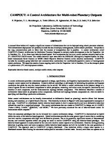
6.1 Simplex implementation Let us introduce the simplex optimziation algorithm (Nelder and Mead, 1965). Consider a compact convex set Ω ⊂ R2 containing the origin. Define a field through a scalar-valued measurement map m : Ω → R and a triangular grid G ∈ Ω as depicted in Figure 5, with aperture d > 0. Introduce an arbitrary point p0 ∈ Ω◦ and a base of vectors given by b1 , b2 such that bT1 b1 = bT2 b2 = d2 and bT1 b2 = d2 cos π/3. The grid is then given by G = {p ∈ Ω| p = p0 + kb1 + ℓb2 , k, ℓ ∈ Z}.
300
300
250
250
200
200
150
150
100
100
50
50
0
0
−50
0
100
200
300
400
500
−50
0
(a) Situation after 6 time steps. 300
250
250
200
200
150
150
100
100
50
50
0
0
0
100
200
300
200
300
400
500
400
500
(b) Situation after 12 time steps.
300
−50
100
400
500
(c) Situation after 18 time steps.
−50
0
100
200
300
(d) Situation after 24 time steps.
Fig. 6. Simplex coordination algorithm executing a search in a noisy quadratic field with drift. A simplex z = (z1 , z2 , z3 ) ∈ G 3 is then defined by three neighboring vertices in G. We suppose, without loss of generality, that V (z3 ) ≥ V (zi ), i = 1, 2. Given a simplex z = (z1 , z2 , z3 ) the next simplex, z ′ , is then generated from z by reflecting z3 with respect to the other vertices, i.e., it is given by the mapping
derive bounds on the distance to the minimizer when the simplex algorithm terminate (Silva et al., 2004)
z 7→ z ′ = f (z) = (z1 , z3 , z1 + z2 − z3 ).
A simulation study was done to illustrate the behavior of the proposed hierarchical control structure. In particular we have considered the simplex search with two AUV’s in a time-varying scalar field, which could represent salinity, temperature, etc. in a region of interest. Figure 6 shows four snapshots of the evolution of the AUV’s. The field is quadratic with additive white noise and a constant drift. As illustrated in the figure, the vehicles are able to find the minimizer of the field.
(6)
The map f defines the way-point generation function g : L → R3 of the team controller, as described in the sequel. Consider a case with two AUV’s: v1 and v2 . (It is easy to incorporate more vehicles.) Suppose the team controller of v1 will control both v1 and v2 , so we have the following assignments according to the definition of TeamController: role(tc1(v1)):=$master; role(tc2(v2)):=$slave;
Note that L(step) denotes the visited location at the last step of the algorithm. If we denote it by z = (z1 , z2 , z3 ), as above, it simply follows that the next location set should be given by z ′ = (z1 , z3 , z1 + z2 − z3 ). This relation defines g. Few theoretical results on the convergence properties of the simplex algorithm exist for functions in Rm with m ≥2. In general, it is not known if the algorithm converges to the minimizer even for smooth fields (Lagarias et al., 1998). It is easy to find examples such that the fixed-size simplex algorithm ends up far from the optimum even for convex quadratic functions, especially if the they have steep valley shapes. For particular fields, such as quadratic fields, one can
6.2 Simulations
REFERENCES de Sousa, J. Borges, A. Girard and K. Hedrick (2004). Safe controller design for intelligent cruise control using differential games. In: Proceedings of the 2004 MTNS conference. Deshpande, A., A. Gollu and L. Semenzato (1997). The shift programming language and run-time system for dynamic networks of hybrid automata. Technical Report UCB-ITS-PRR-97-7. California PATH. Krasovskii, N.N. and A.I. Subbotin (1988). Gametheoretical control problems. Springer-Verlag.
Lagarias, Jeffrey C., James A. Reeds, Margaret H. Wright and Paul E. Wright (1998). Convergence properties of the nedler-mead simplex in low dimensions. SIAM Journal of Optimization 9(1), 112–147. Lewis, E., Ed.) (1989). Principles of Naval Architecture. Society of Naval Architects and Marine Engineers. 2nd revision. Nelder, J.A. and R. Mead (1965). A simplex method for function minimization. Computing Journal 7, 308–313. Silva, Jorge, Alberto Speranzon, J. Borges de Sousa and Karl Henrik Johansson (2004). Hierarchical search strategy for a team of autonomous vehicles. In: Proceedings of the 2004 IAV conference. IFAC.
Appendix A. AN ASIDE ON SHIFT Shift is a specification language for describing networks of hybrid automata. Shift users define types (classes) with continuous and discrete behavior as depicted in table A.1. A simulation starts with an initial set of components that are instantiations of these types. A component is an input-output hybrid automaton. Instances of components have unique names. The world-evolution is derived from the behavior of these components. The inputs and outputs of different comtype Vehicle input output state discrete export flow transition setup }
{ (what we feed to it) (what we see on the outside) (whats internal) (discrete modes of behavior) (event labels seen from the outside) (continuous evolution) (discrete evolution) (actions executed at create time)
Table A.1. Shift component. ponents can be interconnected. Each discrete state has a set of differential equations and algebraic definitions (flow equations) that govern the continuous evolution of numeric variables. These equations are based on numeric variables of this type and outputs of other types accessible through link variables. The transition structure of the hybrid automaton may involve synchronization of pairs or sets of components. The system alternates between the continuous mode, during which the evolution is governed by the flow equations, and the discrete mode, when simulation time is stopped and all possible transitions are taken, as determined by guards and/or by event synchronization among components. During a discrete step components can be created, interconnected, and destroyed. Shift allows hybrid automata to interact through dynamically reconfigurable input/output connections and synchronous composition.