equipped with Atheros AR5212 cards operating in 802.11b mode. The implementation .... Network Parameters,â IEEE Communications Letters, vol. 10, no. 8, pp.
1
A Control Theoretic Approach to Distributed Optimal Configuration of 802.11 WLANs Paul Patras∗† , Albert Banchs∗, Pablo Serrano∗ and Arturo Azcorra∗† ∗ University Carlos III of Madrid, Spain † IMDEA Networks, Madrid, Spain
Abstract—The optimal configuration of the contention parameters of a WLAN depends on the network conditions in terms of number of stations and the traffic they generate. Following this observation, a considerable effort in the literature has been devoted to the design of distributed algorithms that optimally configure the WLAN parameters based on current conditions. In this paper we propose a novel algorithm that, in contrast to previous proposals which are mostly based on heuristics, is sustained by mathematical foundations from multivariable control theory. A key advantage of the algorithm over existing approaches is that it is compliant with the 802.11 standard and can be implemented with current wireless cards without introducing any changes into the hardware or firmware. We study the performance of our proposal by means of theoretical analysis, simulations and a real implementation. Results show that the algorithm substantially outperforms previous approaches in terms of throughput and delay. Index Terms—Wireless LAN, IEEE 802.11, DCF, adaptive MAC, distributed algorithm, multivariable control theory
The approaches proposed so far for the configuration of 802.11 can be classified in the following two groups: • Centralized approaches [4]–[7]. These approaches are based on a single node (the Access Point) that periodically computes the set of MAC layer parameters to be used and signals this configuration to all stations. • Distributed approaches [8]–[11]. With these approaches, each station independently computes its own configuration. Among other advantages, this removes the signaling overhead and naturally fits the ad-hoc mode of operation of 802.11 which uses no Access Point. In this paper we propose a novel distributed algorithm, based on control theory, that adaptively adjusts the CW configuration of the WLAN with the goal of maximizing the overall performance. The key advantages of the proposed algorithm over existing distributed approaches are: The proposed algorithm is sustained by mathematical foundations from the multivariable control theory field that guarantee convergence and stability while ensuring a quick reaction to changes. In contrast, most of the previous proposals are based on heuristics that lack these foundations. • Our mechanism is standard-compliant and can be implemented with existing hardware. In contrast, the existing proposals change the 802.11 mechanism, which introduces additional complexity and requires modifying the hardware and/or firmware of existing wireless cards. • In contrast to all previous proposals, which modify the contention parameters of all stations upon congestion, our algorithm only acts on those stations that are contributing to congestion; as a result, it provides stations that are not contributing to congestion with a better delay performance. The rest of the paper is organized as follows. In Section II we summarize the 802.11 DCF mechanism. Section III presents the proposed algorithm. In Section IV we conduct a steady state analysis of the WLAN to derive the optimal collision probability that maximizes performance (which is used as the reference signal of our control system). In Section V we perform a control theoretic analysis of the system and based on this analysis we configure the controller parameters to guarantee a proper tradeoff between stability and speed of reaction to changes. Section VI validates the algorithm by means of simulations, and Section VII presents a prototype that proves the algorithm can be implemented with •
I. I NTRODUCTION The throughput performance of the DCF mechanism of 802.11 Wireless LANs (WLANs) depends on the number of active stations and the Contention Window (CW ) with which they contend. If too many stations use too small CW ’s, then the collision rate will be very high and consequently throughput performance will be low. Similarly, if few stations contend with too large CW ’s, the attempt rate will be low and the channel will be underutilized most of the time, yielding a poor throughput performance also in this case. In line with this explanation, many works in the literature (e.g. [1], [2]) have shown that, given a number of actively contending stations, there exists an optimal CW configuration that maximizes the throughput performance. The CW configuration used by the 802.11 standard [3] is statically set, independently of the number of contending stations. As a result, it does not provide optimal performance. In particular, standard 802.11 stations contend with overly small CW ’s, which yields a degraded performance as the number of contending stations in the WLAN increases. In order to avoid this undesirable behavior, many schemes have been proposed in the literature to dynamically adapt the CW to the current WLAN conditions. Although the various mechanisms differ in the details, their common aim is to adjust the CW configuration to the optimal value corresponding to the number of currently active stations and thereby maximize the WLAN throughput performance.
2
current hardware. Section VIII reviews related work and finally Section IX concludes the paper.
station 1 +
II. IEEE 802.11 DCF In this section we briefly summarize the 802.11 DCF mechanism [3]. With DCF, a station with a new frame to transmit senses the channel. If this remains idle for a period of time equal to the DCF interframe space parameter (DIF S), the station transmits. Otherwise, if the channel is detected busy, the station monitors the channel until it is measured idle for a DIF S time, and then executes a backoff process. When the backoff process starts, the station computes a random number uniformly distributed in the range (0, CW − 1), and initializes its backoff time counter with this value. CW is called the contention window and for the first transmission attempt the minimum value (CWmin ) is used. In case of a collision CW is doubled, up to a maximum value CWmax . As long as the channel is sensed idle, the backoff time counter is decremented once every time slot Te . When a transmission is detected on the channel, the backoff time counter is “frozen”, and reactivated after the channel is sensed idle. When the backoff time counter reaches zero, the station transmits its frame in the next time slot. A collision occurs when two or more stations start transmitting simultaneously. An acknowledgment (Ack) frame is used to notify the transmitting station that the frame has been successfully received. If the Ack is not received within a given timeout, the station reschedules the transmission by reentering the backoff process. After a failed attempt, all the retransmissions of the same frame are sent with the retry flag set. If the number of failed attempts reaches a predetermined retry limit, the frame is discarded. Once the backoff process is completed, CW is set again to CWmin . As it can be seen from the above description, the behavior of a station depends on the CWmin and CWmax parameters. In the revised version of the standard [12], which incorporates the mechanisms defined in 802.11e [13], these are configurable parameters that can be set to different values for different stations. The rest of the paper is devoted to the design of a standard compliant mechanism for the optimal setting of the above parameters. In order to benefit from the features of the binary exponential backoff algorithm, we set CWmax = 2m CWmin , taking the m value of the default configuration (which is m = 6 in IEEE 802.11g), and concentrate on adaptively adjusting the CWmin parameter. III. DAC A LGORITHM In this section we present the proposed algorithm, hereafter referred to as Distributed Adaptive Control (DAC) algorithm. DAC adjusts the CWmin parameter of each station with the goal of driving the WLAN to the optimal point of operation. To achieve the above goal, DAC uses a classical system from multivariable control theory [14] which is shown in Fig. 1. In this system, each station runs an independent controller that gives the CWmin value to be used by the station. In this paper we have chosen to use a well known controller from
2pothers,1 – pown,1
+
e1 -
PI controller
CWmin,1
pcol
WLAN
2pothers,n – pown,n
+
+
en -
PI controller
CWmin,n
pcol station n
Fig. 1.
DAC Algorithm
classical control theory, namely a proportional-integral (PI) controller. As it can be seen from Fig. 1, the PI controller of station i takes as input the error signal ei and gives as output the CWmin,i configuration of the station. The choice of the error signal ei is a critical part of the design of the DAC algorithm, as it drives the system behavior both under steady and transient conditions. In steady conditions, a key requirement for the choice of ei is that there exists a single stable point of operation that yields optimal performance. This requirement is analyzed in Section IV, which shows that the system reaches the optimal point of operation by driving the collision probability to a desired value. In transient conditions, we set the following requirements when choosing the error signal: i) When the collision probability is far from its desired value, the error signal needs to be large in order to trigger a quick reaction towards the desired value. ii) When the collision probability is around its desired value but stations do not share bandwidth fairly, the error should also be large in order to achieve a fair bandwidth sharing. iii) In case of congestion, only the saturated stations1 ) should increase their CWmin,i , thus avoiding that the nonsaturated stations (which are not contributing to congestion) are unnecessarily penalized. In order to satisfy the above requirements, we take the error signal as the sum of two terms. The first one is: ecollision,i = pothers,i − pcol
(1)
where pothers,i is the probability that a transmission of a station different from i collides and pcol is the desired value for the collision probability. This term ensures that if the WLAN is operating at a different collision probability from the desired one, the error is large, achieving thus the first of the three requirements stated above. 1 Following [1], with saturated station we refer to a station that always has packets ready for transmission.
3
The second term of the error signal is: ef airness,i = pothers,i − pown,i
(2)
where pown,i is the probability that a transmission of station i collides. This term ensures that if two stations do not share the bandwidth fairly due to having different CWmin,i ’s, the error will be large. Indeed, a station with a small CWmin,i transmits with a large probability, and therefore its pothers,i will be larger than pown,i , yielding a large ef airness,i . This fulfills the second requirement. Additionally, the ef airness,i term also ensures that in case of congestion only the saturated stations increase their CWmin,i , which yields the last of the requirements stated above. This is caused by the fact that saturated stations have a larger transmission probability; as a result, their pothers,i is larger and their pown,i smaller, which makes their ef airness,i larger. The combination of Eqs. (1) and (2) yields the following error signal: ei
= =
ecollision,i + ef airness,i 2pothers,i − pown,i − pcol
(3)
where, as depicted in Fig. 1, the term 2pothers,i − pown,i corresponds to the feedback signal measured from the WLAN and pcol is the reference signal, whose value is given in Section IV. Having chosen the error signal as given by the above expression, the remaining key challenge for its computation is the measurement of the values of pown,i and pothers,i . In particular, the challenge lies in measuring these values by using only functionality available in current wireless cards. To achieve this, we proceed as follows. To compute the own collision probability at station i, pown,i , we take advantage of the following statistics which are readily available from wireless cards: the number of successful transmission attempts, denoted by T , and the number of unsuccessful attempts, F . pown,i is then computed by applying the following formula F (4) F +T The probability pothers,i cannot be computed following the above procedure since with current hardware it is not possible to measure the unsuccessful attempts of other stations. Instead, we compute pothers,i by looking at the retry flag of the frames successfully transmitted observed by station i. Let S be the number of frames with the retry bit unset, and R be the number of frames with the retry bit set. Then, if we assume that no frames are discarded due to reaching the retry limit, the collision probability pothers,i can be computed as pown,i =
R (5) pothers,i = R+S With the above, each station i periodically measures pothers,i and pown,i and computes the error signal ei from these measurements. This error signal is then fed into the controller which triggers an update of CWmin,i . As a safeguard against too large and too small values of CWmin , when updating CWmin,i we force that it can neither take
values below a given lower bound nor above an upper bound. In particular, the values that we have chosen for the lower and upper bounds in this paper are the default CWmin and CWmax values used by the DCF standard (with the 802.11g physical layer, these are 16 and 1024, respectively). Regarding the frequency with which the CWmin,i is updated, in this paper we choose to update it every beacon interval, by triggering the algorithm upon the reception of a beacon frame. The key advantages of this choice are: •
•
It ensures compatibility with existing hardware, since WLAN cards conforming to the IEEE 802.11 revised standard are able to update the configuration of the CWmin parameter at the beacon frequency. It is a simple way to ensure that all the stations update their configuration with the same frequency.
As an exception to the above, if the number of samples used to compute pothers,i or pown,i at the moment of receiving the beacon frame is smaller than 20, the update is not triggered but deferred until the next beacon. The reason is to avoid that a too small number of samples induces a high degree of inaccuracy in the estimation of these parameters. In what follows, we assume that there are always enough samples available and updates are never deferred. From the above description of DAC, it can be seen that the algorithm relies on pcol as well as the parameters of the PI controller (namely Kp and Ki ) [15]. The following two sections address the issue of properly configuring these parameters. IV. S TEADY S TATE A NALYSIS In the following we analyze the DAC algorithm under steady conditions and, based on this analysis, we compute the value of the pcol parameter that maximizes the throughput obtained in steady state. The analyses of this and the following section assume saturation conditions, while the simulation results presented in Section VI also cover the non-saturated case. To analyze the system under steady conditions, we proceed as follows. Since the controller includes an integrator, this ensures that there is no steady state error [15]. The steady solution can therefore be obtained from imposing ei = 0 ∀i
(6)
2pothers,i − pown,i − pcol = 0
(7)
from which
Let τi be the probability that station i transmits at a given slot time [1]. pown,i and pothers,i can be computed as a function of the τi ’s as follows. pown,i is the probability that a transmission of station i collides � pown,i = 1 − (1 − τk ) (8) k�=i
pothers,i is the average collision probability of the other stations measured by station i, which is computed by adding
4
the individual collision probabilities of the other stations weighted by their transmission probability ⎛ ⎞ � � τk ⎝1 − � pothers,i = (1 − τl )⎠ (9) l�=i τl k�=i
E
Controller
CWmin
System
l�=k
By using the above expressions for pothers,i and pown,i , we can express Eq. (7) as a system of equations on the τi ’s. Theorem 12 guarantees the uniqueness of this system of equations and shows that all stations have the same transmission probability in the steady state solution: τi = τj ∀i, j
(10)
Note that the above result given by Theorem 1 is of particular importance since it guarantees the existence of a unique stable point of operation for the system. Indeed, while the existence of a unique point of operation can be easily guaranteed in a centralized system by imposing the same configuration for all stations, it is much harder to guarantee this in a distributed system in which each station chooses its own configuration. Substituting τi = τ , given by Eq. (10), into Eqs. (7), (8) and (9) yields (11) pcol = 1 − (1 − τ )n−1 From the above equation, it follows that by setting the pcol parameter in our control system, we fix the conditional collision probability under steady conditions. In the following, we analyze how this parameter should be set in order to maximize the throughput of the WLAN. The throughput obtained by a station in a saturated WLAN can be computed as follows
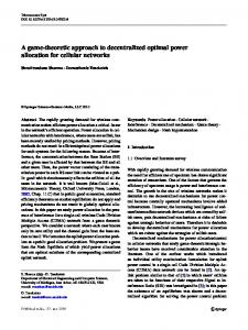
Fig. 2.
Control system
From the above, we have that under optimal operation the conditional collision probability in the WLAN, pcol , is a constant independent of the number of stations. The fact that pcol is constant is a key result of our analysis, since it allows us to configure this parameter to a fixed value independent of the WLAN conditions. V. S TABILITY A NALYSIS We next conduct a stability analysis of DAC and, based on this analysis, we compute the configuration of the Kp and Ki parameters of the PI controller. The DAC system presented in Fig. 1 can be expressed in the form of Fig. 2, where ⎞ ⎛ CWmin,1 ⎟ ⎜ .. CWmin = ⎝ (19) ⎠ . CWmin,n and
⎞ ⎛ ⎞ e1 2pothers,1 − pown,1 − pcol ⎟ ⎜ ⎟ ⎜ .. E = ⎝ ... ⎠ = ⎝ ⎠ . en 2pothers,n − pown,n − pcol ⎛
(20)
Ps l (12) Ps Ts + Pc Tc + Pe Te where l is the average packet length, and Ts , Tc and Te are the duration of a success, a collision and an empty slot time, respectively, and Ps , Pc and Pe are the respective probabilities,
Our control system consists of one PI controller in each station i that takes ei as input and gives CWmin,i as output. Following this, we can express the relationship between E and CWmin as follows
Ps = nτ (1 − τ )n−1
(13)
CWmin (z) = C · E(z)
Pe = (1 − τ )n
(14)
Pc = 1 − nτ (1 − τ )n−1 − (1 − τ )n
(15)
r=
Following the analysis of [6], it can be seen that the total WLAN throughput is maximized with the following approximate expression for the optimal τ , 1 2Te τopt ≈ (16) n Tc With the above τopt , the corresponding optimal conditional collision probability is equal to
�n−1 1 2Te n−1 pcol = 1 − (1 − τopt ) =1− 1− (17) n Tc which can be approximated by pcol ≈ 1 − e 2 The
−
2Te Tc
theorems and their proofs are included in the Appendix.
(18)
where
⎛
⎜ ⎜ ⎜ C=⎜ ⎜ ⎝
CP I (z) 0 0 0 CP I (z) 0 0 0 CP I (z) .. .. .. . . . 0 0 0
... ... ... .. .
(21) 0 0 0 .. .
⎞ ⎟ ⎟ ⎟ ⎟ (22) ⎟ ⎠
. . . CP I (z)
with CP I (z) being the z transform of a PI controller Ki (23) z−1 In order to analyze our system from a control theoretic standpoint, we need to characterize the Wireless LAN system with a transfer function that takes CWmin as input and gives the E as output. Since the probabilities pothers,i and pown,i are measured every 100 ms interval, we can assume that the obtained measurements correspond to stationary conditions and therefore the system does not have any memory. With this assumption, CP I (z) = Kp +
5
E can be computed from the CWmin,i ’s with Eq. (20), where pown,i and pothers,i are computed as a function of the τi ’s following Eqs. (8) and (9). Furthermore, the τi ’s can be calculated as a function of the CWmin,i ’s from the following nonlinear equation [1], τi =
2 1 + CWmin,i (1 + pown,i
�m−1 k=0
(2pown,i )k )
and
(33)
From the above, (n − 3)(1 − τopt )n−2 ∂ei = ∂τj (n − 1)
(24)
where pown,i is a function of τi as given by Eq. (8). The above equations give a nonlinear relationship between E and CWmin . In order to express this relationship as a transfer function, we linearize this relationship when the system suffers small perturbations around its stable point of operation. A similar approach was used in [16] to analyze RED from a control theoretical standpoint, although the analysis of [16] focused on a single-variable system while we analyze a multivariable system. In the following, we study the linearized model and force that it is stable. Note that the stability of the linearized model guarantees that our system is locally stable [16]. We express the perturbations around the point of operation as follows:
∂pown,i = (1 − τopt )n−2 ∂τj
(34)
Following a similar procedure we obtain ∂ei = 2(1 − τopt )n−2 ∂τi Combining all the above, ⎛ n−3 2 n−1 ⎜ n−3 2 ⎜ n−1 ⎜ n−3 n−3 H = KH ⎜ ⎜ n−1 n−1 .. ⎜ .. ⎝ . . n−3 n−1
n−3 n−1
n−3 n−1 n−3 n−1
2 .. .
... ... ... .. .
n−3 n−1
...
(35)
n−3 n−1 n−3 n−1 n−3 n−1
.. . 2
⎞ ⎟ ⎟ ⎟ ⎟ ⎟ ⎟ ⎠
(36)
where
where CWmin,i,opt is the CWmin,i value that yields the transmission probability τopt given by Eq. (16). With the above, the perturbations suffered by E can be approximated by
� � �m 1 + pcol k=0 (2pcol )k (37) 2 With the above, we have our system fully characterized by the matrices C and H. The next step is to configure the Kp and Ki parameters of this system. Following Theorem 2, we have that as long as the {Kp , Ki } setting meets the following condition the system is guaranteed to be stable:
δE = H · δCWmin
−(n−1)KH (Kp −Ki )−1 < (n−1)KH (Kp −Ki )+1 (38)
CWmin,i = CWmin,i,opt + δCWmin,i
where
⎛
⎜ ⎜ H=⎜ ⎜ ⎝
∂e1 ∂CWmin,1 ∂e2 ∂CWmin,1
∂e1 ∂CWmin,2 ∂e2 ∂CWmin,2
∂en ∂CWmin,1
∂en ∂CWmin,2
.. .
.. .
... ... .. . ...
(25)
(26) ∂e1 ∂CWmin,n ∂e2 ∂CWmin,n
.. .
∂en ∂CWmin,n
⎞ ⎟ ⎟ ⎟ ⎟ ⎠
(27)
The above partial derivatives can be computed as ∂ei ∂τj ∂ei = ∂CWmin,j ∂τj ∂CWmin,j where from Eq. (24) we have � � �m 1 + pown,j k=0 (2pown,j )k ∂τj = −τj2 ∂CWmin,j 2
(28)
Kp = 0.4Ku
(39)
Kp 0.85Ti
(40)
and Ki =
In order to compute Ku we proceed as follows. From Eq. (38) with Ki = 0 we have Kp
1 − k�=i,j
Combining the above with Eq. (52), we have the the second term of Eq. (52) is surely negative, which forces the first term to be 0. Thus, τi = τj (56) which proves the second part of the theorem. To proof uniqueness of the solution, we proceed as follows. From the above we have τi = τ ∀i
=
(52)
Substituting the expressions of pown,j and pown,i by Eq. (8) and operating on the above yields ⎞ ⎛ � � � τk 1 − τk − 1 − τk − pcol ⎠ = 0 (τj − τi ) ⎝1 −
(58)
Since the lhs of the above equation decreases from 1 to 0 with τ while the rhs is a constant between 0 and 1, we have that there exists a unique τ value that resolves the above equation. From Eq. (57) it further follows that the only solution to the system is τi = τ ∀i. The proof follows.
(49)
k�=i
� τ � k�=i l k�=j τl
Substituting this into Eq. (48) yields
(57)
P1 (z) (z 2 + a1 z + a2 )(z 2 + a�1 z + a�2 )
(64)
P2 (z) + a1 z + a2 )(z 2 + a�1 z + a�2 )
(65)
and b=
(z 2
where P1 (z) and P2 (z) are polynomials and a1 = −(n − 1)KH Kp − 1
(66)
a2 = (n − 1)KH (Kp − Ki ) � � n−3 � a1 = − 2 − KH Kp − 1 n−1 � � n−3 � a2 = 2 − KH (Kp − Ki ) n−1
(67) (68) (69)
According to Theorem 3.5 of [14], a sufficient condition for the stability of a transfer function is that the zeros of its pole
12
polynomial (which is the least common denominator of all the minors of the transfer function matrix) fall within the unit circle. Applying this theorem to (I + CH)−1 C yields that the roots of the polynomials z 2 + a1 z + a2 and z 2 + a�1 z + a�2 have to fall inside the unit circle. This can be ensured by choosing coefficients {a1 , a2 } and {a�1 , a�2 } that belong to the stability triangle [19]: (70) a2 < 1 a1 < a2 + 1
(71)
a1 > −1 − a2
(72)
a�2 < 1
(73)
a�2
(74)
and a�1
−1 − a�2
(75)
Eqs. (70), (72), (73) and (75) are satisfied for any {Kp , Ki } setting. If Eq. (71) is satisfied, then Eq. (74) is also satisfied. Therefore, it is enough to guarantee that Eq. (71) is met. The proof follows. Corollary 1. The Kp and Ki configuration given by Eqs. (46) and (47) is stable. Proof: It is easy to see that Eqs. (46) and (47) meet the condition of Theorem 2.