Optimal Allocation of Testing Effort: A Control Theoretic Approach

Proceedings of the 4th National Conference; INDIACom-2010 Computing For Nation Development, February 25 – 26, 2010 Bharati Vidyapeeth’s Institute of Computer Applications and Management, New Delhi

Optimal Allocation of Testing Effort: A Control Theoretic Approach P.K. Kapur1 Udayan Chanda2 Vijay Kumar3 Department of Operational Research, University of Delhi, Delhi-110007 Email: [email protected]; [email protected]; [email protected] ABSTRACT Allocation of financial budget to a software development project during the testing phase is a staggering task for software managers. The challenges become stiffer when the nature of the development process is considered in the dynamic environment. Many software reliability growth models (SRGM) have been proposed in last decade to minimize the total testing-effort expenditures but mostly under static assumption. The main purpose of this paper is to investigate an optimal resource allocation plan to minimize the cost of software during the testing and operational phase under dynamic condition. An elaborate optimization policy based on the optimal control theory is proposed and numerical examples are illustrated. The paper also studies the optimal resource allocation problems for various conditions by examining the behavior of the model parameters. The experimental results greatly help us to identify the contributions of each selected parameter and its weight. KEYWORD SRGM, Testing Effort Allocation, Optimal Control Theory, Learning Curve Effect. 1. INTRODUCTION The development cycle is a challenging but significant component of any SDLC project. The challenges become stiffer when the nature of the development process is considered in the dynamic environment. In general companies installed different project management tools to synchronize the process with all other components of project. Software is released to the users phase at the end of the testing phase of Software Development Life Cycle (SDLC). With larger development and testing efforts, better quality software can be ensured. But this would be time consuming and is undesirable in the prevalent competitive market conditions. Allocation of financial budget to a software development project during the testing phase in the dynamic environment is a critical decision that a software manager’s has to make. During testing, resources such as manpower and time (computer time) are consumed. The failure (fault identification) and removal are dependent upon the nature and amount of resources spent. Many software reliability growth models have been proposed in last decade to minimize the total testing-effort expenditures but mostly under the assumptions that the relationship between the testing effort consumption and testing time (the calendar time) follows Exponential and Rayleigh distribution. The time dependent behavior of the testing effort has been studied earlier by Basili et al [1], Huang [5], Putman [16] and Yamada

et al. [19]. Exponential curve is used if the testing resources are uniformly consumed with respect to the testing time and Rayleigh curve otherwise. Logistic and Weibull type functions have also been used to describe testing effort. Another approach is due to Musa et al. [11], where they have assumed the resource consumption as an explicit function of number of faults removed and calendar time. Kapur et al. [10] have discussed the optimization problem of allocating testing resources in software having modular structure. And proposed that allocation of testing effort should depend upon the size and severity of faults and also suggested that for different resource constraints one can develop a trade-off between the maximum number of faults to be removed in each module and the effort required. In the research paper the authors have proposed three different MTEFs (Marginal Testing Effort Functions) for the optimization problem. As discussed, over the last couple of decades many software reliability growth models (SRGM) have been proposed to minimize the total testing-effort expenditures, but mostly under static assumption. Here in this paper we have tried to investigate an optimal resource allocation plan to minimize the cost of software during the testing phase under dynamic condition. The paper also studies the optimal resource allocation problems for various conditions by examining the behavior of the model parameters. 2. CONTRIBUTION OF STUDY A Software Reliability Growth Model (SRGM) explains the time dependent behavior of fault removal. Several SRGMs have been proposed in software reliability literature under set of assumptions and testing environment, yet more are being proposed. The proposed SRGM in this paper takes into account the time dependent variation in testing effort. The testing efforts (resources) that govern the pace of testing for almost all the software projects are [11] : a) Manpower which includes  Failure identification personnel  Failure correction personnel. b) Computer time. The key function of manpower engaged in software testing is to run test cases and compare the test results with desired specifications. Any departure from the specifications is termed as a failure. On a failure the fault causing it is identified and then removed by failure correction personnel. The computer facilities represent the computer time, which is necessary for failure identification and correction. The influence of testing effort has also been included in some SRGMs [5,6,7,8,9,10,16

Optimal Allocation of Testing Effort: A Control Theoretic Approach

and 18]. In 1976, Myers proposed that software system should be constructed and tested in separate in sequential step. Yamada et al. [19], Hou et al. [4], Pham and Zhang [14] has recommended that system-level software testing occurred only after the system was completely developed. Recently, Blackburn et al. [2] however suggested that software construction and system debugging and testing should be viewed as concurrent activities. Kapur and Bardhan [8] explored the relationship between the number of faults removed with respect to time and/or testing effort. The authors propose that since during the testing phase of a software development cycle, faults are removed in two phases: first a failure occurs, and then the fault causing that failure is corrected hence the testing effort should be spent on two separate processes; failure identification and fault removal. In there paper the authors developed a SRGM incorporating time lag not only between the two phases but also through the segregation of resources between them and proposed two alternate methods for controlling the testing effort for achieving desired reliability or error detection level. Chiang and Mookerjee [3] analyze a development process in which system integration occurs when the number of errors in the system reaches a certain threshold. In this paper we propose an alternate rationale for optimal allocation of testing resources using learning curve phenomenon under dynamic environment. The article is divided into the following sections: model development, dynamic optimization, theoretical results, special cases and numerical analysis. Finally, the article concludes with a discussion on the application, extension and limitations of the model. 3. MODEL DEVELOPMENT Software industry is the high technology industry where innovation and knowledge creation forms the primary fuel for continued firm growth. The innovation-related factors like development process, software testing & debugging process and team structure have significant impact on a firm’s future growth potential. In the last few decades the world of new software development based on sophisticated development method, new technologies and adapt tools has evolved rapidly due to the intensified market competition. Software has become an integral part of nearly every engineered product and fuel for controlling various systems such as manufacturing processes, public transportation etc. At the same time the threat due to software failure is also becoming more intensified. As the criticality of these applications grows, the importance of delivering systems with high reliability cannot be overemphasized. To ensure reliability, software testing is necessary. In this research paper, we recommend that software testing and debugging should be viewed as concurrent activities. Our goal is to build a simple, structured model of concurrent testing and debugging with a view to gaining insights. In the paper, we have assumed that during the testing phase of a Software development Life Cycle (SDLC), the fixed total resources ( W ) at any point of time ‘ t ’can be divided into two portions ‘ w1 t  ’ and ‘ w2 t  ’

(where, w1 t  is the current effort consumption to fix fault at

time ‘ t ’ and w2 t  is the current effort consumption due to testing at time ‘ t ’) as depicted in the figure 1. Total Resources Utilized during the Software Development Life Cycle at any point of time ‘t’ is ‘W’ (before release)

Resources allocated for debugging the software during the Software Development Life Cycle at any point of time ‘t’

Resources allocated for testing of the software during the Software Development Life Cycle at any point of time ‘t’

‘w 1 (t)’ (before release)

‘w 2 (t)’ (before release)

Figure 1: Allocation of Total resources To solve the dynamic optimization problems for resource allocation, we have used optimal control theory approach and assumed that software testing and debugging can run concomitantly. The control variable here ‘ w1 t  ’ and ‘ w2 t  ’ manages the evolution of a system in such a way that an optimal outcome (here, minimum cost) is achieved by the end of the time horizon. In the paper the relation between failure rates of software and cost to decrease this rate is modeled by various types of learning curves effect. 4. DYNAMIC OPTIMIZATION PROBLEM We begin our analysis by stating a general model with a very few assumptions. We are restricting our analysis to the case of a firm that controls its resources for testing and debugging under finite planning horizon. We are also consistent with the idea that the latent faults in the software system are detected and eliminated during the testing phase and the number of faults remaining in the software system gradually decreases as the testing progresses. Therefore, it is reasonable to assume the following differential equation:

xt  

d m(t )  bw1 t a  mt  dt

(1)

where, xt  is the number of fault removed at time ‘ t ’.

mt  is the cumulative number of fault removed till time ‘ t ’. ‘ a ’ is the initial fault content. ‘ b ’ is the detection rate.

Apart from the above notations few other notations are also used in the analysis, they are as follows: T : the planning period. c1 mt , w1 t  : Total cost per unit at time ‘ t ’ for cumulative fault removed mt  and debugging effort w1 t  .

c 2 is the cost of testing per unit testing efforts.

Proceedings of the 4th National Conference; INDIACom-2010

W

 2 c1 c1 and c1w1w1  w1 w12

is the total resources utilized during the Software Development Life Cycle at any point of time ‘ t ’.

where, c1w1 

Now suppose the software firm wants to minimize the total expenditure over the finite planning horizon T . Then the objective function for the company can be given by

From the above optimality conditions, we can get the following results:

T

min

 c1 t xt   c2 w2 t dt 0

(7)

subject to xt  

dmt   xb, w1 t  dt

and, (2)

where m0   0 and w1 t   w2 t   W

5. OPTIMAL SOLUTION To solve the problem, Maximum principle can be applied. The current value Hamiltonian is as follows [17]:

  c1 t    t xt   c 2 w2 t 

   c1 t    t   c2   w2 t   W    ct 1w t  ba  mt    ct 1w t   1 1     (8) Integrating equation (4) with the transversility condition, we have the future cost of removing one more fault can be given as

w1 t ; w2 t   0

H  c1 t xt   c 2 w2 t    t xt 

   c1 t    t   c2   w1 t     ct 1w t  ba  mt    ct 1w t   1 1    

T

t

(3)

where,  t  is the current value adjoint variables (shadow cost of xt  ) which satisfy the following differential equation.

 c d dH x (4)  (t )       1 x   c1    dm dt m m with the transversality condition at t  T ,  T   0

We can interpret  t  as the marginal value of faults at time ‘ t ’, which should be negative because increasing the number of faults will increase the debugging cost. The physical interpretation of the Hamiltonian H can be given as follows:  t  stands for future cost incurred as one more fault introduced in the system (at time t ). Thus the Hamiltonian is the sum of current cost c1 x and the future cost x . In short, H represents the instantaneous total cost of the firm at time t. The following is the necessary condition hold for an optimal solution:

H  0  c1w1 bw1 a  m   c 2  c1   ba  m  w1

(5) Other optimality conditions is

 2H   c1w1w1 x  2c1w1 x w1  c1   x w1w1   0 w12 (6)

 c1 t  xt   xt   c1 t    t  dt mt    mt 

 (t )   

(9)

6. THEORETICAL RESULTS The general formulation and characteristics of the proposed model will help in gaining some insight into important factors influencing the optimal policies. Now taking time derivative on (7), we have



    xw1  c1xw1m1   x xc1w1m1  xmc1w1  c1mxw1  xw1m1   w1   c1w1w1 x  2c1w1 xw1  c1  xw1w1







(10) From (10) depending on the sign of numerator, we have the following three cases:’ case1. when     xw1  c1xw1m1   x xc1w1m1  xmc1w1  c1m xw1  xw1m1   (11) w1 t  will be monotonically increasing.





Case 2.



    x w1  c1 x w1m1   x xc1w1m1  x m c1w1  c1m x w1  x w1m1  

w1 t  will be monotonically decreasing.



(12)

Case 3.



    x w1  c1 x w1m1   x xc1w1m1  x m c1w1  c1m x w1  x w1m1  

w1 t  will attain saturation point.

(13)



Optimal Allocation of Testing Effort: A Control Theoretic Approach

Now,

6.1. Special Cases In general at the initial level during the testing phase of the software development lifecycle the debugging costs confine the large chunk of development cost due to uncertain nature of the errors. Later on as the potential fault content reduces the cost due testing captures the majority of the expenditure. By this we can assume that the debugging cost gradually decreases with time. In this section we have considered two scenarios to depict the cost of debugging on the optimal policies of the control variable.

Hamiltonian. Thus, w1 t  can be given as

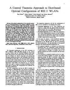
Case 1. In this section we are assuming that the total cost per unit for cumulative fault removed at time ‘ t ’ is constant. i.e. c1 t   c1 (14)

W if H w1  0   w1 t   undefined if H w1  0  if H w1  0 0

For constant fault removal function, the objective function can be written as T

min

 c xt   c w t dt 1

2

H w1  ( c1   ) x w1  c 2    c1 ba  m   c 2 (20)

From (20), it is clear that the Hamiltonian is linear in control variable w1 t  , we have the following bang–bang and

singular solution form for w1 t 

w1* (t )

2

W if (  c1 )b(a  m)  c 2   undefined if (  c1 )b(a  m)  c 2 0 if (  c1 )b(a  m)  c 2  (22)

(15)

Hence,

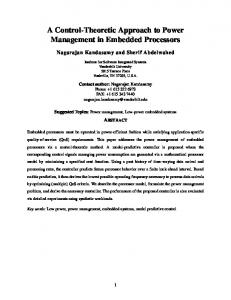
w2 (t )

w1 t ; w2 t   0

0 if (  c1 )b(a  m)  c 2   undefined if (  c1 )b(a  m)  c 2 W if (  c )b(a  m)  c 1 2  (23)

w1 t 

And the corresponding Hamiltonian can be given as

H t   c1   t xt   c 2 W  w1 t    c1   t ba  mt   c 2 w1  c 2W

(21)

i.e.

0

subject to dmt  xt    xb, w1 t  dt where m0   0 and w1 t   w2 t   W

to maximize the

(16)

W

And, the adjoint variable  t  can be defined as  d  (t )   t   bw1 (t )(c1   t ) dt

(17)

with the transversality condition at t  T ,  T   0 From (17) and the transversality condition of  T  , we have

Figure2: Allocation policy for Debugging Effort

T

 (t )   bw1 (t )(c1 (t )   (t ))dt

(18)

t

The necessary condition for optimality is

H w1  0

c2

(19)

Proceedings of the 4th National Conference; INDIACom-2010

 mc t    t   w2 t   W  xt  1  c2  

w2 t 

(29)

If the planning horizon is long enough and debugging cost function follows learning curve phenomenon, then from (28) and (29) we have the following two general allocation strategies

W

Policy 1. For, the case in which mc1     c 2 i.e. when the cost of per unit testing is much less than the debugging cost, then the optimal allocation path of debugging effort will monotonically increases and the testing effort path monotonically decreases over time (see figure 4).

c2 Figure3: Allocation policy for Testing Effort

Case 2 In this section we have considered a cost function that follows learning effect phenomenon (Pegels 1969), which is of the form

c1 w1 t , mt   c0 w1 t 

m t 1

(24)

where, c 0 is the base cost. For this case, the Hamiltonian can be defined as:

H   c1 t    t xt   c 2 w  w1 t 

(25)

Thus for optimality the necessary condition is

H w1  c1w1 x   c1   xw1  c2  0

(26)

Here, c1w1 

(27)

x c1 m  1 and xw1  w1 w1

Thus,

 mc t    t   w1 t   xt  1  c2  

(28)

The physical interpretation of the above equation is that the optimal policy for fixing effort is equal to the ratio of total cost of fixing per unit bugs to per unit testing cost multiplied by the number of errors removed at time ‘ t ’. Hence, the optimal policy for w2 t  can be expressed as:

w1 t 

Effort

The physical interpretation of the above optimal policies for effort allocation can be given as:  If the total cost of fixing a bug is less than the unit testing cost, then invest all the efforts for debugging purpose only.  On the other hand if per unit fixing cost becomes greater than the testing cost, then invest whole effort on testing

w2 t  Time

Figure 4: Allocation policies for the two Efforts when

mc1     c 2

This result can also be visualized as a situation when most of the faults are identified during a certain time point of the testing phase of SDLC and not much testing are required henceforth. Hence to fix the faults at the earliest, the software firm may consider increasing the debugging effort. For the optimal testing effort, as the higher portion of the faults are identified hence company may keep it low for sometime. Policy 2. For, the case in which mc1     c 2 i.e. when the cost of debugging is less than the testing cost, then the optimal allocation path of debugging effort will monotonically decreases and the testing effort path monotonically increases over time (see figure 5).

Optimal Allocation of Testing Effort: A Control Theoretic Approach

w1 t 

w1=0.7

100 Cumulative Number of Fault Removed

Effort

w2 t 

w1=0.6 w1=0.5

90 80

w1=0.4

70 w1=0.3

60 50 40 30 20 10

Time

21

20

19

18

17

16

15

14

13

12

11

9

10

8

7

6

5

4

3

2

1

0 Time

Figure 5: Allocation policies for the two Efforts when

mc1     c 2

Figure 6: Cumulative Number of Faults Removed vs. Time 300

a  1000  0   40 c 2  400

b  0.4 x0  2

w1 0  0.3 c 0  1000

In this analysis, the objective is to check the significance of allocation of debugging effort ( w1 ), hence its value has been assumed to be constant throughout the product life cycle. In the analysis it has been seen that as the value of w1 is gradually increased keeping the other parameters constant, the rate of fault removal increases rapidly and the cost due to future removal slows down remarkably. This situation may arise, when the majority of the faults were identified during the testing and hence larger effort on debugging can accelerate the fault removal rate. At the same time it will reduces any cost for future removal.

250 Shadow Cost (Adjoint Variable)

7. NUMERICAL ANALYSIS In this section, the property of the various optimal policies has been described on the proposed model using numerical example. The purpose of this study is to get some insight into the result and also to study the impact of change in efforts on the debugging cost model and the corresponding optimal cost model. Several simulation runs were conducted using various parameter values; results converged quickly and were stable. To do so, we have considered the Pegels (1969) form of learning curve to define the debugging function. First some base values were considered and then different model parameters are varied individually. The base values are as follows:

w1=0.7 200 150 100

w1=0.6 w1=0.5 w1=0.4

50

w1=0.3

0 1 2 3 4 5 6 7 8 9 10 11 12 13 14 15 16 17 18 19 20 21 -50 Time

Figure 7: Shadow Cost vs. Time Analysis was also performed to examine the trend in the debugging cost. The result indicates that increasing the debugging effort ( w1 ) will reduces the total debugging cost and at same time it reduces the rate of increase of the total expenditure. These patterns were revealed throughout the numerical analysis. 8. CONCLUDING REMARKS In this paper we have studied an optimal resource allocation plan to minimize the cost of software during the testing and operational phase under dynamic condition. Using optimal control theoretic approach we have obtained number of policies for fixing effort and testing effort for different cost function. We observed that when cost are constants the optimal policy for expenditure on fixing effort is to allocate the resources on debugging only if the total cost of fixing a bug is less than the unit testing cost. If per unit fixing cost becomes greater than the testing cost in the absence of any debugging effort, then invest whole effort on testing. Similar kind of interpretation can be drawn from other optimal solutions. Continued on Page No. 438

Proceedings of the 4th National Conference; INDIACom-2010

Continued from Page No. 430 The theoretical results obtained here confirm that the optimality conditions as described in previous literature. Many additional useful results have also been identified. The results were verified using simulation technique. 9. FUTURE SCOPE A few limitations in our approach that suggests areas for future research, are as follows. The model is based on the assumption that at any point of time the total resources allocated for debugging and testing is fixed, as a result both the variable (i.e. testing and debugging) becomes explicitly interdependent. Hence controlling one variable will automatically control the other. But in practice they may not be explicitly interdependent. Also, it is been considered that the cost function depends on only one state function (i.e. fault removal function) hence the model ignores the other stages of fault removal process (i.e. detection). The rate of detection can heavily be influenced by the correction process. Thus, there is need to incorporate explicitly the other dimensions of fault detection and removals clearly. Incorporating other state variables (i.e. dimensions viz detection function) can be areas of future research. Finally, the model can be extended in several ways, e.g. by incorporating other kind of software reliability growth models (e.g. S-shaped) in the optimization modelling framework that can be useful to gain insights into the worthiness of allocation of resources in software reliability analysis. 10. REFERENCE [1] Basili, V.R. and M.V. Zelkowitz (1979), Analyzing medium scale software development, in Proceedings of the 3rd International Conference on Software Engineering, 116-123. [2] Blackburn, J. D., G. D. Scudder, L. N. Van Wassenhove. (2000). Concurrent software development. Comm. ACM 43(11) 200–214. [3] Chiang, I. R., V. S. Mookerjee. (2004). A fault threshold policy to manage software development projects. Inform. Systems Res. 15(1) 3–19. [4] Hou, R. H., S. Y. Kuo, Y. P. Chang. (1997). Optimal release times for software systems with scheduled delivery time based on the HGDM. IEEE Trans. Comput. 46(2) 216–221. [5] Huang, C-Y, S-Y. Kuo and J.Y. Chen (1997), Analysis of a software reliability growth model with logistic testing effort function, Proceeding of 8th International Symposium on software reliability engineering, 378-388. [6] Ichimori, T., S. Yamada and M. Nishiwaki (1993), Optimal allocation policies for testing-resource based on a Software Reliability Growth Model, Proceedings of the Australia –Japan workshop on stochastic models in engineering, technology and management, 182-189.

[7] Kapur P.K., R.B. Garg and S. Kumar (1999), Contributions to Hardware and Software Reliability, World Scientific, Singapore. [8] Kapur P K, Bardhan AK. (2002). Testing Effort Control through Software Reliability Growth Modelling. International Journal of Modelling and Simulation, 22(1): 90-96. [9] Kapur PK, Gupta Anu, Shatnawi Omar and Yadavalli V.S.S. (2006). Testing effort Control using Flexible Software Reliability Growth Model with Change point. International Journal of Performability Engineering, 2(3): 245-262. [10] Kapur P.K., Bardhan A.K., Yadavalli VSS (2007). On allocation of resources during testing phase of a modular software. International Journal of Systems Science, 38 (6): 493 - 499. [11] Musa, J.D., Iannino, A. and Okumoto, K. (1987), Software reliability: Measurement, Prediction, Applications, Mc Graw Hill, New York. [12] Myers, G. J. (1976). Software Reliability: Principles and Practices. John Wiley & Sons, New York. [13] Pegels, C.C. (1969). On startup or learning curves: An expected view, AIIE Trans, 7(4): 216-222. [14] Pham, H., X. Zhang. (1999). A software cost model with warranty and risk costs. IEEE Trans. Comput. 48(1): 71– 75. [15] Pillai, K. and Nair, V.S.S. (1997), A Model for Software Development effort and Cost Estimation. IEEE Transactions on Software Engineering; 23(8), 485-497. [16] Putnam, L (1978), A general empirical solution to the macro software sizing and estimating problem, IEEE Transactions on Software Engineering SE-4, 345-361. [17] Sethi SP, Thompson GL. (2005). Optimal Control Theory – Applications to Management Science and Economics, 2nd Edn. Springer, New York. [18] Xie M. (1991), Software reliability modeling, World Scientific, Singapore. [19] Yamada, S., J. Hishitani and S. Osaki (1993), Software Reliability Growth Model with Weibull testing effort: A model and application, IEEE Trans. on Reliability R-42, 100-105.