A Convective Wake Parameterization Scheme for Use ... - AMS Journals

456

MONTHLY WEATHER REVIEW

VOLUME 126

A Convective Wake Parameterization Scheme for Use in General Circulation Models LIYING QIAN, GEORGE S. YOUNG,

AND

WILLIAM M. FRANK

Department of Meteorology, The Pennsylvania State University, University Park, Pennsylvania (Manuscript received 18 September 1996, in final form 16 May 1997) ABSTRACT In the atmosphere, the cold, dry, precipitation-driven downdrafts from deep convection spread laterally after striking the surface, inhibiting new convection in the disturbed wake (cold pool) area. In contrast, the leading edge of this cold air lifts unstable environmental air helping to trigger new convection. A GCM cannot resolve the disturbed and undisturbed regions explicitly, so some parameterizations of these critical mesoscale phenomena are needed. The simplest approaches are to either instantly mix downdraft air with the environment, or instantly recover the downdraft air. The instant-mixing approach tends to lead to unrealistic pulsing of convection in environments that would otherwise be able to support long-lived mesoscale convective systems while the instant recovery approach usually overestimates surface energy fluxes. By replacing these simplistic approaches with a physically based convective wake–gust front model, these problems are substantially remedied. The model produced realistic parameterized wakes that closely resemble those observed in the Global Atmospheric Research Program’s Atlantic Tropical Experiment and Tropical Ocean and Global Atmosphere Coupled Ocean–Atmosphere Response Experiment when given reasonable inputs based on observations taken during these experiments. For realistic downdraft characteristics, wake recovery time is on the order of hours, which is significantly different from the instant recovery or instant mixing assumed in previous parameterizations. A preliminary test in midlatitude continental conditions also produced reasonable wake characteristics. Sensitivity tests show the model sensitivities to variations in downdraft mass flux, downdraft thermodynamic characteristics, and surface wind/downdraft traveling velocity. Prognostic studies using a simple coupled cloud model successfully simulated the convective termination due to stabilization of the boundary layer by precipitation-driven downdrafts, the initiation of convection after the boundary layer recovery by surface fluxes, and the phenomenon of surface flux enhancement during the convective phase.

1. Introduction Successful simulations of the global circulation require accurate parameterizations of subgrid-scale processes. The parameterizations of deep (precipitating) convection, atmospheric boundary layer processes, and surface processes are crucial physical processes parameterized in general circulation models (GCMs). These processes are highly interactive, and one major problem that limits the accuracy of their parameterizations in GCMs is that most models do not resolve important interactions among deep convection, boundary layer processes, and surface processes. To address this problem, we introduce a simple convective wake–gust front model that is suitable for use in most GCMs regardless of their type of convective parameterization scheme. Deep (precipitating) convection generally occurs when convectively unstable air within or just above the boundary layer rises in cumulonimbus updrafts of order 1–10-km diameter (e.g., LeMone and Zipser 1980),

Corresponding author address: Dr. Liying Qian, Department of Meteorology, The Pennsylvania State University, 503 Walker Building, University Park, PA 16802-5013. E-mail: [email protected]

q 1998 American Meteorological Society

warming the free atmosphere and replacing the boundary layer air with cooler and usually drier air from aloft. In most convective regimes, the low-level air that feeds the convection is only marginally unstable such that a decrease in its equivalent potential temperature of only a few degrees would eliminate its convective instability (Emanuel 1994). Therefore, a GCM cumulus parameterization scheme is typically very sensitive to the thermodynamics of the air that is assumed to be the source of the convective updrafts. Most deep convection is organized on the mesoscale, with much of it occurring in mesoscale convective systems (MCSs) (e.g., Houze and Betts 1981; Chen et al. 1996). An individual MCS is typically too small to be resolved explicitly by a GCM, so the effects of both the MCS itself and the embedded convection must be parameterized. A widely accepted schematic of a typical MCS (in this case a tropical cloud line system) is shown in Fig. 1 (Zipser 1977). Regardless of the exact organization of the convection within an MCS, one important feature that they all have in common is a pool of relatively cold (and usually dry) air detrained into the boundary layer from convective downdrafts that reach the surface. Because the air within this ‘‘wake’’ region is denser than the undisturbed air outside the pool, the

FEBRUARY 1998

QIAN ET AL.

457

FIG. 1. Schematic of a class of squall system (Zipser 1977).

cold air spreads as a gravity current. The moving boundary between the advancing cold air and the environment is referred to as the ‘‘gust front.’’ In Fig. 1, the gust front is being maintained by downdrafts located to the rear side of the cloud line, while new updrafts are forming from the undisturbed environmental air as it is lifted along the sloping gust front. Because a convective wake region only occasionally fills an area corresponding to the grid size of a GCM, most of the time the boundary layer of a convective region is not resolved accurately by the conventional, nonpartitioned models, which have only one value of each state variable at each vertical level in the grid column. Such a model continually mixes downdraft air from the convective parameterization with the existing air in the boundary layer, cooling and drying the low levels uniformly, while in nature the undisturbed portions of the boundary layer would retain values of temperature and moisture close to their values prior to the time step. Note that in Fig. 1 the convection is feeding off undisturbed air, which has quite different thermodynamic properties than the convective wake air or any mixture of the wake and undisturbed areas. Because deep convection tends to be very sensitive to relatively small variations in boundary layer temperature and moisture, failure to resolve the separation of the bound-

ary layer into disturbed and undisturbed regions will cause the convection to shut off prematurely in a grid column as well as affect the simulated cloud properties. (While some of the simpler cumulus parameterizations do not attempt to simulate the effects of downdrafts, this simplification results in even greater inaccuracies in the representation of convection.) Failure to resolve the convective wake–gust front portion of a grid column also tends to result in underestimation of surface fluxes within a GCM. In nature, the mesoscale circulations occurring within an area equivalent to that of a typical GCM grid column would be expected to produce negative correlations between air temperature and winds at the surface (e.g., Ledvina et al. 1993). These unresolved correlations would result in a greater upward sensible heat flux at the surface than would be predicted from parameterizations that used grid-scale variables alone to compute the flux. Often, there is also an upward enhancement of the surface latent heat flux due to subgrid-scale processes. These unresolved fluxes are thought to be of major importance in understanding coupling between the atmosphere and ocean, and a major goal of the Tropical Ocean and Global Atmosphere Coupled Ocean–Atmosphere Response Experiment (TOGA COARE) was to improve parameterization of these processes (Webster and Lukas 1992).

458


VOLUME 126

The convective wake–gust front model discussed below is designed to partition the boundary layer of each convectively active GCM grid column into convectively disturbed and undisturbed portions. It utilizes the mass flux and properties of convective downdrafts predicted by a cumulus parameterization scheme to initiate and maintain a cold wake region, with the boundaries of the assumed rectangular wake moving as gravity currents. The model predicts the movements of the wake boundaries, the depth of the wake, the surface fluxes within the wake and the environment, and the recovery of the wake to environmental conditions using a simple and economical procedure. This information is then used to predict the total surface fluxes of heat and moisture in the GCM and to provide information to the cumulus parameterization, such as the thermodynamic properties of the updraft air, the height to which undisturbed air is lifted by the gust front, and an estimate of the total mass lifted by this mesoscale process. Section 2 describes the convective wake–gust front model (hereafter wake model) formulation, and section 3 presents results of preliminary tests of this model under both tropical maritime and midlatitude continental conditions, a series of sensitivity experiments showing the characteristics of the model’s behavior and illustrating its utility in GCM simulations, and simple prognostic tests. Conclusions are presented in section 4. 2. Model formulation As shown in Fig. 1, the precipitation-driven downdrafts from deep convection spread out after striking the ground and form a convective wake that can extend up to several hundred kilometers to the rear of the squall line (Johnson and Nicholls 1983). The cold and dry air inhibits the growth of new deep convection within the wake, while the gust front that separates the wake from the preconvective environment lifts the potentially buoyant environment boundary layer air to initiate or enhance deep convection. Most other classes of MCS exhibit the same basic relationships between wake and convection although configuration may vary significantly. The formulation described herein is based on these relations and so captures the key processes in most classes of MCS. The exact geometric configuration modeled in this paper closely resembles the most studied class, the squall line. Some special convective systems, such as low-precipitation- (LP) type supercell thunderstorms, depart from this conceptual model and so would not be well represented by this formulation. Because it is designed for GCMs, some small-scale effects, such as terrain effects, are also ignored in this formulation. The scheme models the evolution of the dimensions and thermodynamic properties of the convective wake and the dimensions and intensity of the gust front updrafts. For simplicity, the model described below approximates the temperature and moisture structure of the wake as vertically well mixed, constant in the along-squall di-

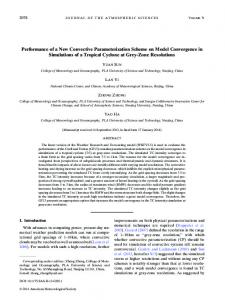
FIG. 2. Schematic of a convective wake: (a) dimensions of the wake, (b) the assumed linear variation of temperature along the wake age dimension, and (c) same as (b) but for water vapor mixing ratio.

rection, and linearly varying in the wake-age (front-torear) dimension. The modeled wake also has a spatially uniform depth that varies temporally with the downdraft mass flux into the wake; the propagation speed of front, rear, and sides of the wake; and the wake recovery processes. The wake takes a rectangular shape with the front of the wake being the side nearest where the convective downdrafts detrain. A schematic of a convective wake is shown in Fig. 2. The depth of the ‘‘head,’’ the narrow region of enhanced depth along the leading edge, is estimated differently, as discussed later. The main processes that affect the wake evolution are downdraft mass flux, gravity current propagation, surface fluxes, and entrainment fluxes at the top of the wake. The gravity current propagation of the convective downdraft surface outflow acts to increase the wake area and decrease the wake depth. The area increase is described as 1 ]a 5 [(Vf 1 Vr )L 1 2Vs W ], ]t A

(1)

FEBRUARY 1998

459

QIAN ET AL.

where a is the fractional area covered by the wake within a grid box, A is the grid-box area, L denotes the distance the wake extends behind the squall line’s gust front (i.e., length), W denotes the width of the wake’s leading edge, and V f , V r , and V s are the propagation speeds of the front, rear, and sides of the wake, respectively. Simpson (1969), Charba (1972, 1974), and Addis (1984) found that the propagation of the gust front is well described by gravity current theory in a calm environment. It has also been recognized that strong interaction exists between gust fronts and ambient flow (Simpson and Britter 1980; Chen 1995; Liu and Moncrieff 1996). Simpson and Britter (1980) conducted laboratory experiments to study the effect of uniform ambient flow on gust fronts and found that uniform ambient flow affects gust fronts linearly. Environmental shear, however, affects gust fronts in a more complicated way (Chen 1995; Liu and Moncrieff 1996). We will ignore the interaction of the gust front with the environmental shear profile until quantitative results are available. Therefore, the outflow propagation speeds (V f , V s , V r ) are calculated from the gravity current speeds (V gf , V gs , V gr ), which are in turn calculated from the depth and density characteristics of the wake. The modification of propagation speed due to ambient wind is calculated following Simpson and Britter (1980), and we only consider the modifications to the wake front and rear speed (i.e., the sides are perpendicular to the ambient wind). Because the traveling speed of the downdrafts affects the propagation speed at the front of the wake, we made an adjustment to the speed of the wake’s front V f based on the horizontal traveling speed of the convective downdraft (V d ) (Lucero 1983). Assigning the direction of the density current motion of the wake front to be the x-axis direction, we have

!

Z (u 2 uyi)g Vgi 5 k k ye , u yi

m d 5 rA

](aZ k ) , ]t

(3)

where m d is the downdraft mass flux at the top of the wake (assumed to be known from the cumulus parameterization) and r is the mean air density within the wake. Rearranging this equation permits the calculation of the change in Z k with time:

1

2

]Z k 1 ]a 5 m d 2 rZ k A . ]t raA ]t

u

n21

5

u n21 1 u rn21 f , 2

Vr 5 2Vgr 1 0.62U e (2)

where uy e is the virtual potential temperature of the environment, and uy i is the virtual potential temperature of the relevant side of the wake. The value k is the internal Froude number, which is a constant with a value of order 1 (Charba 1974, 1.25; Mitchell and Hovermale 1977, 0.52–0.73; Droegemeier and Wilhelmson 1987, 0.75). Simpson (1969) recommended k 5 0.78 based on their laboratory studies and other laboratory studies. In this paper, we set k 5 0.78. Here, Z k is the depth of the wake, U e is the wake ambient wind, and V d is the downdraft horizontal traveling velocity. Velocity V d is assumed to be the mean cloud-layer wind, which is calculated from the mean cloud-layer wind vector (Merritt

(5)

where subscripts f and r denote the front and rear of the wake, respectively. Assuming that heat content is conserved during the process of detrainment of downdrafts to the wake, we obtain the mean potential temperature at time step n (present time step) to be m Dtu 1 rA(a n21 Z n21 )u k u 5 d d m dDt 1 r(a n21 Z n21 )A k

Vs 5 Vgs

(4)

For both temperature and moisture, the initiation value at the front of the wake is computed following each injection of downdraft air in order to maintain the observed linear distribution along the age (i.e., wake length) dimension while conserving heat and moisture. The mean potential temperature of the wake at time step n 2 1 is

n

i 5 f, r, s

Vf 5 max[(Vgf 1 0.26Vd ), Vd ] 1 0.62U e ,

1985). The virtual potential temperatures uy e and uy i are determined by the downdraft mass feeding and the wake recovery formulation as discussed later in this section. When the sides of the wake reach the edges of the grid column, V s is set to zero and the wake is assumed to become two-dimensional. The downdraft mass flux effect on Z k is computed from mass conservation. The wake mass budget equation is

n21

,

(6)

where Dt is the time step, u d is the potential temperature of the downdraft at the top of the wake, and r is the mean density of the wake. Further, assuming that the rear potential temperature does not change during the process of detrainment of downdrafts to the wake

u nr 5 u rn21,

(7)

we then get the front-side temperature due to the detrainment of downdrafts to be n

u nf 5 2 u 2 u n21 . r

(8)

Thus, by knowing the mean potential temperature (net heat content) of the wake and the potential temperature at the recovery edge of the wake, one can compute the wake front potential temperature, which preserves the linear temperature distribution across the wake. The lowest temperature is at the front because the downdraft mass flux feeding occurs there, and the highest tem-

460


VOLUME 126

perature is at the rear because of wake recovery. Some lateral mixing within the wake is implicit in this step for all but very special conditions. Moisture is treated in the same way. Because the wake propagates as a gravity current, the wake recovery is defined by virtual potential temperature rather than solely by temperature or moisture. The air near the rear of the wake is assumed to recover when its virtual potential temperature equals or exceeds the virtual potential temperature of the air in the undisturbed environment. This procedure is described below. The surface flux effects on wake recovery are diagnosed using the bulk aerodynamic approximation. The surface sensible and latent heat fluxes at any position x within the wake are

which introduces some implicit lateral mixing. The entrainment fluxes at position x are

rC p (w9T9)sfc,x 5 2rC p C h U x (T x 2 Tsfc )

where (w9u9)sfc and (w9q9)sfc are surface fluxes integrated horizontally across the wake, and (w9u9) zk and (w9q9) zk are the corresponding integrated entrainment fluxes. Some lateral mixing is implicit in this equation since it is assumed that the temporal derivatives of temperature and mixing ratio are uniform across the wake. Following these computations, the rear of the wake is located at the x value where the new virtual potential temperature equals that of the environment. The recovered part of the wake between this point and the old rear is mixed with the environmental boundary layer air. As long as the wake area does not exceed a specified fraction of the grid-box area (acrit , assumed to be 0.9 in this study), all interactions between the grid box and its neighbors are assumed to take place with the environmental air. If the wake area exceeds this fraction, the wake is assumed to dominate. The wake air is then instantaneously mixed with the remaining environment air via area-weighted average to form a new, uniform environment, and boundary layer convection is allowed throughout the grid box. Similarly, if the average temperature in a wake increases to within 0.5 K (an arbitrary threshold) of the environmental temperature, the wake is eliminated and mixed with the environment via this weighted-average procedure. The equations above do not form a closed parameterization scheme unless the initial wake dimensions and thermodynamic characteristics are specified. The assumptions used in this specification are 1) the wake takes a square shape at its initial formation and 2) the wake reaches an equilibrium at the end of the first time step, which requires that the rate of volume spreading by the resulting gravity current equals the downdraft mass flux. These two assumptions and mass conservation result in the following equations valid for the first time step:

rL(w9q9)sfc,x 5 2rLC h U x (q x 2 qsfc ),

(9)

where the subscripts x and sfc denote the front-to-rear positions, within the wake and the surface, respectively; C h is the bulk transfer coefficient for heat and moisture; and U x is the surface layer wind speed at position x. Here, Tsfc and qsfc are the sea surface temperature and its corresponding saturation water vapor mixing ratio. The value of U x is determined based on two assumptions: 1) the surface wind at front and rear are composed of their respective density current speed and the ambient flow (Simpson and Britter 1980), and 2) surface wind varies linearly across the wake. The values of T x and q x are also obtained from the assumed linear variations of temperature and moisture within the wake. The parameterization of the wake top entrainment flux effect on the wake is based on the mixed-layer theory of Deardorff (1972, 1974), Betts (1973), and Tennekes (1973). The surface buoyancy flux at any position x within the wake is calculated following Stull (1988): (w9u9y )sfc,x 5 (w9u9)sfc,x (1 1 0.61q) 1 0.61 u(w9q9)sfc,x , (10) where the averaged mixing ratio q and potential temperature u across the wake are used instead of q x and u x to simplify computations. This simplification is reasonable because the magnitudes of variations of mixing ratio and temperature across the wake are far smaller than those of surface fluxes based on the bulk aerodynamic estimations of surface fluxes. The top buoyancy flux and the entrainment velocity at position x is then (w9u9) y z k , x 5 20.2(w9u9) y sfc,x Wx 5

1 dt 2 5 2 dZ k

x

(w9u9) y zk , x , (Du y ) x

(11)

where(Duy ) x is the virtual potential temperature jump at position x at the top of the wake. An integrated entrainment velocity across the wake is obtained from the above equation to update the wake depth uniformly,

(w9q9) zk , x 5 2W x (Dq) x (w9u9) zk , x 5 2W x (Du) x ,

(12)

where (Dq) x and (Du) x are water vapor mixing ratio and potential temperature jumps at position x at the top of the wake. The heating and moistening caused by the vertical flux convergence within the wake are therefore (w9T9)sfc 2 (w9u9) zk ]u 5 ]t Zk (w9q9)sfc 2 (w9q9) zk ]q 5 , ]t Zk

(13)

L5W Z k (2L 1 2W)V 5

md r

m dDt 5 rZ k LW,

(14)

FEBRUARY 1998

where V is the gravity current speed, r is the wake density, and both are computed from the downdraft thermodynamic characteristics. The values Z k , L, and W are the wake dimensions at the end of the first time step. These three equations can be solved for the three wake dimensions. Once convection has been initiated, most new convection is triggered by the gust front updrafts (Zipser 1977). Thus, it is important to estimate the size and vertical velocity of the updrafts along the gust front as well as the height to which the air is lifted. Under many conditions, only the coldest side of the wake will actually have strong enough updrafts to trigger deep convection. Therefore, for efficiency, we assume that only the coldest side, the front of the wake, will trigger deep convection. Some MCSs, however, do not trigger deep convection only on one side. For this kind of MCSs, the scheme should be modified at this point to be most applicable. The maximum updraft velocity at the top of the gust front’s head (W g ) is calculated following Simpson (1969, 1972) and Young and Johnson (1984). The results of Simpson (1969, 1972) and Young and Johnson (1984) are obtained in a calm environment; therefore, we modify their results to include the effects of environmental wind: W g 5 g(V f 2 U e ),

(15)

where g is a constant with a value on the order of 0.5 (Young and Johnson 1984). Simpson’s laboratory results in 1969 and 1972 give a range of 0.4–0.6. The level at which this velocity occurs is the depth of the cold-pool head (Z h ). This value is the same as the wake depth (Z k ) for slowly moving downdraft sources V d K V f , but Z h becomes significantly greater than Z k for faster moving systems. As V d increases still further, Z h reduces once again to approximately Z k for V d . 2Vf . The formula for Z h is derived from the results of the doctoral dissertation of Lucero (1983): 

Z k Zh 5

461

QIAN ET AL.





11 1 0.62V 2 , Vd

Vd , 2Vf

f

(16) Vd . 2Vf .

Z k ,

The diameter of the cumulus triggered by the gust front should either be set to the width (d u ) of the gust front updraft or to some spectrum which has a median of this width: d u 5 KZ k ,

(17)

where K is a constant of order 1. The case studies of Young and Johnson (1984) and Shapiro (1984) suggest the values of 1.5 and 0.5 to 1.0, respectively. The current paper does not make use of d u , but it is an important parameter in some cumulus parameterizations.

TABLE 1. Specified downdraft, boundary layer environment, and sea surface conditions for typical tropical convection.

Precipitation-driven downdraft Environment Sea surface

Temperature (K)

Water vapor mixing ratio (g kg21)

298.0 301.0 302.0

18.0 20.0 24.9*

* Surface saturation water vapor mixing ratio at T 5 302.0 K; Usfc 5 5 m s21, Vd 5 7 m s21, Zi 5 600 m.

3. Results a. Overall success of system in parameterizing wake processes 1) SIMULATIONS

WITH TYPICAL TROPICAL

CONDITIONS

Convective wakes, especially those induced by mesoscale convective systems, are an important phenomenon in the Tropics, as demonstrated during the Global Atmospheric Research Program Atlantic Tropical Experiment (GATE) (Betts 1976; Mandics and Hall 1976; Zipser 1977; Gaynor and Ropelewski 1979; Houze and Betts 1981) and TOGA COARE (Young et al. 1995). Gaynor and Mandics (1979) found that within the tropical eastern Atlantic region during GATE, downdraftmodified boundary layers (or wakes) accompanying precipitating convective systems covered approximately 30% of the total area on the average, and in these wakes, cool convective downdraft air produced shallow, 100– 300-m-deep mixed layers over large areas and recovered only slowly over a period of 2–10 h. By using squallline data from GATE, Johnson and Nicholls (1983) found that immediately behind the 200-km-wide squall line to a distance of about 100 km existed a very cool, stable layer of air several hundred meters deep just above the ocean surface, and surface temperature and specific humidity within the squall-line wake were as low as 48C and 3 g kg21 below the surrounding environmental values. In this preliminary test, a representative dataset (Table 1) based on GATE and TOGA COARE observations is used to provide model initial values to evaluate the wake model’s performance in this regime. The model domain (i.e., one grid cell) is 300 km 3 300 km, and the time step is 40 min (all of the following model runs have the same domain and time step). The downdraft mass flux is chosen to be constant with M d 5 0.5 3 10 9 kg s21 for the entire length of the run (16-h simulation). Assuming convective downdraft vertical velocities to be on the order of 21 m s21 at cloud base (Emmitt 1978; LeMone and Zipser 1980), we will get around 1% fractional area covered by convection for this amount of downdraft mass flux. For the calculation of entrainment fluxes at the top of the wake, we specify the thermodynamic properties just above the top of the wake the same as the large-scale sounding of this grid column. Failure to distinguish the anvil-in-

462


VOLUME 126

FIG. 3. Properties of a parameterized wake under typical tropical maritime conditions.

duced stable layer from the environmental capping inversion via partitioning of the free atmosphere into disturbed and undisturbed regions simplifies the model greatly but has a negative impact on wake-model performance, as we will see later in this section. The thermodynamic property jumps at the top of the environmental mixed layer are specified to be Duy ù 0.2 K, Du 5 1.3 K, and Dq 5 26 g kg21 , which are typical of tropical fair-weather conditions (Sarachik 1974). Under this specification and from the mixed-layer data in Table 1, the potential temperature and water vapor mixing ratio over the mixed layer (both the wake and the environment) are 302.3 K and 14.0 g kg21 , respectively. Some characteristics of the parameterized wake are shown in Fig. 3. The wake area reaches a steady-state value of around 30% of the grid box (Fig. 3a), which corresponds to an extended length of the wake of around 90 km (Fig. 3c). The wake depth ranges from 200 to 400 m, while the wake head is almost two times deeper than the wake body at the beginning. Later on, the surface heat flux recovery process reduces the virtual temperature contrast between the wake and the environment. This decrease causes the density current speed to decrease until it is much smaller than the downdraft source velocity [i.e., the downdraft overtakes the gust front—(16)], and the head depth gradually drops to match the wake depth. Figure 3d shows the virtual potential temperatures of the environment and the wake front. The virtual potential temperature of the wake front is more than 2 K lower than the environment. The features of the parameterized wake show the consistency with the observations cited above. Figure 4 illustrates a process of wake formation and

gradual recovery at a fixed point that experienced 40 min of convective rainfall. With the rainfall (thus the convective downdraft) onset, the air becomes much cooler and drier, and a wake is formed. Thereafter, the air temperature and moisture within the wake gradually increase because of the surface fluxes. Young et al. (1995) documented comprehensively the initiation and recovery process of composite TOGA COARE wakes. Because the data of temperature, water vapor mixing ratio, and wind velocity in Table 1 are based on their paper, a comparison to their results is favored. Figure 5 shows the formation and recovery of wake air temperature, water vapor mixing ratio, and virtual temperature adapted from their paper. It is obvious that the evolution of air temperature and virtual temperature of the modeled wake are in close agreement with the observations. Both the temperature and virtual temperature drop more than 28 with the wake onset and then recover gradually. The mixing ratio of the modeled wake, however, recovers much more rapidly than that observed by Young et al. (1995). Zipser (1977) and Houze and Betts (1981) also observed that the moisture within a wake recovers more slowly than the temperature. The reason is that the entrainment moisture flux through the boundary between a wake and the overlying anvil-induced dry stable layer could be larger than surface evaporation flux, and the entrainment fluxes act to retard the wake recovery. However, in the present model, we did not distinguish the thermodynamic characteristics of the anvil-induced stable layer from the environmental capping inversion. The mixing ratio of this stable layer should be much lower than that of the environment. Therefore, entrainment flux of moisture is underestimated. As a

FEBRUARY 1998

FIG. 4. Variations of air temperature, water vapor mixing ratio, and virtual temperature during a life cycle of a simulated tropic wake.

result, the modeled moisture recovery process is quite rapid (Fig. 4b). This indicates that the parameterization of an anvil-induced stable layer in a GCM is important as well and should be incorporated into GCM parameterizations via a model of comparable sophistication to this wake model. The life cycle of the modeled wake is around 6 h as defined by the virtual potential temperature. In nature, such a cycle for MCSs can be longer. The life cycle of the composite TOGA COARE wake of Young et al. (1995) is 12 h on average. 2) SIMULATIONS

463

QIAN ET AL.

WITH SIMPLIFIED MIDLATITUDE

CONDITIONS

The preliminary tests of the wake model for midlatitude continental conditions could be rather complicated because of the intricacies of the land surface thermodynamic conditions. Therefore we did a greatly simplified test as described below. We deal with the surface sensible and latent heat fluxes instead of the land surface temperature and moisture. Moreover, we ignore the di-

FIG. 5. Variations of air temperature, water vapor mixing ratio, and virtual temperature during a life cycle of the composite TOGA COARE wake (adapted from Young et al. 1995).

urnal variations to retain some modicum of simplicity. According to Oke (1987), the land surface evaporation fraction is

g5

LE , Rn

(18)

where LE is the surface latent heat flux and R n is the surface net radiation flux. The value of g typically ranges from 0.1 to 0.9 when soil goes from dry to wet. According to the surface energy balance, we have R n 5 LE 1 SH 1 G,

(19)

where SH is the surface sensible heat flux and G is the soil energy storage. The above formulas allow us to approximate the surface sensible and latent heat fluxes in both the environment area and wake area by making the following assumptions: 1) assuming the environment is cloudy and therefore the surface net radiation flux in the environment and wake area is uniformly 100 W m22 , 2)

464


VOLUME 126

tropical squall line. The convective surface outflow layer is about 500 m thick. This simulation, although under greatly simplified condition, suggests that the model simulate the midlatitude wake properly. b. Sensitivity studies

FIG. 6. Evolution of wake fractional area and depth during a 16-h simulation under midlatitude continental conditions.

The density current propagation speed and the fluxdriven recovery of the wake determine the area and depth of the wake, which in turn control the area of the wake-stabilized boundary layer and the properties of the gust front–triggered updrafts. Based on these physics, we expect the downdraft characteristics and boundary layer wind to have profound influences on the wake. The sensitivity tests discussed in this section are designed to test the parameterization’s sensitivities to the specified downdraft mass flux, downdraft thermodynamic characteristics, and surface wind/downdraft traveling velocity. The control case is chosen to have the features of M d 5 0.5 3 10 9 kg s21 , T d 5 298.0 K, q d 5 18.0 g kg21 , and Usfc 5 5 m s21 , and the same environmental and surface thermodynamic characteristics as those in the above tropical maritime preliminary test. The downdraft traveling velocity is assumed to be 2 m s21 faster than the surface wind. The solid lines in Fig. 7 show the results of this control case.

the evaporation fraction is 0.3 for the environment area and 0.9 for the wake area, and 3) the soil energy storage is 10% of the surface net radiation flux. The obtained surface-sensible and latent heat fluxes in the environment area are, respectively, 60 W m22 and 30 W m22 , and they are 0 W m22 and 90 W m22 in the wake area. The environmental initial temperature and water vapor mixing ratio are set to 297 K and 12 g kg21 , and the boundary layer depth is assumed to be 1500 m. The temperature and mixing ratio difference between downdraft and environment are assumed to be 7 K and 2 g kg21 , respectively. The downdraft mass flux is specified to be 0.5 3 10 9 kg s21 . The environmental surface wind speed is specified to be 5 m s21 and downdraft traveling velocity to be 7 m s21 , as in the tropical maritime case. Figure 6 shows the wake produced during the 16-h simulation. The wake fills the whole grid box after around 6 h and mixes with the environment. This process is repeated because of the constant downdraft mass flux. The wake area grows rapidly for two reasons: 1) the wake boundaries propagate very rapidly because of the large temperature difference between downdraft and environment, and 2) the wake does not recover significantly during the simulation period because there is no surface sensible heat flux, and the latent heat flux is very small. The wake depth is around 200 m and the head depth is around 350 m. Ogura and Liou (1979) analyzed the structure of a midlatitude squall line in central Oklahoma and found the structure of the squall line exhibits remarkable similarities with the typical

1) Experiment 1. In this test, the downdraft mass flux is reduced by half compared to the control case. The dashed lines in Fig. 7 show the results of this test. The wake is shallower (Fig. 7c) because of the reduced downdraft mass flux. The wake area (Fig. 7a) is considerably reduced, partly due to the slower propagation of gravity current [Eq. (2)], partly due to the early domination by the wake recovery process (wake area and length stop increasing, Figs. 7a and 7b); correspondingly, the wake length is reduced greatly (Fig. 7b). A very significant feature in Fig. 7d is that the wake head depth crashes much earlier. The reason is that the front density current speed in the half mass flux case is smaller, while the downdraft traveling velocity is the same in both cases. Consequently, the downdraft source speed exceeds the density current speed at an earlier stage in the wake life cycle. 2) Experiment 2. Surface wind plays an important role in determining surface fluxes. In this test, the surface wind speed is reduced to 3.5 m s21 , and the downdraft traveling velocity is reduced to 5.5 m s21 correspondingly. The dashed–dotted lines in Fig. 7 show the results of this test. Because of the reduced surface fluxes, the wake recovery process is slower than in the control case, eventually increasing the wake area (Fig. 7a) and the length (Fig. 7b). As a result, the wake is shallower (Fig. 7c). The wake head never crashes (Fig. 7d) because the downdraft traveling velocity is slower and thus the downdraft never overtakes the wake head.

FEBRUARY 1998

QIAN ET AL.

465

FIG. 7. Sensitivity tests to input parameters. Solid lines: control case; dashed lines: sensitivity to downdraft mass flux; dashed–dotted lines: sensitivity to surface wind/downdraft traveling velocity; dotted lines: sensitivity to downdraft thermodynamic properties.

3) Experiment 3. In this test, both the temperature and moisture of the downdraft are increased compared to the control case. The temperature and mixing ratio are 299.5 K and 19.5 g kg21 , respectively. Being less dense, the wake propagates more slowly. Therefore, both the area and length are reduced (Figs. 7a and 7b) and the downdraft overtakes the wake much earlier (Fig. 7d). With the same amount of downdraft mass flux but a smaller area, the wake is deeper (Fig. 7c). 4) Experiment 4. It has been noticed that the internal Froude number has a large range of values (Mahoney 1988). This variability may be attributed to the different environmental conditions (e.g., orography) of gust fronts, different interpretations of the theoretical formulation for the calculation of k, etc. Figure 8 shows the model sensitivities to the Froude number k. Figure 8a indicates that initially, wake fractional area increases with the increase of k because a larger Froude number causes larger propagation speed [Eq. (2)]. According to mass conservation, the wake depth decreases with the increase of a Froude number at the beginning (Fig. 8c). Figure 8c also shows that the wake depth maintains this trend later on. The wake fractional area, however, reverses its initial trend. The reason is that the wake is shallower with a larger Froude number, and consequently, more

wake is recovered with a larger Froude number [Eq. (13)]. The wake length follows the same trends as the wake fractional area by the same reasons. Figure 8d indicates that with a Froude number of 1.25, the wake head does not crash to match the wake depth because of the large propagation speed of the wake front. The sensitivity test illustrates that the model has some sensitivity to k, and k should be estimated carefully. One remaining internal parameter is K in (17). It is an important parameter in some cumulus parameterization in that it plays a role in determining the updraft mass flux triggered by the gust front. The sensitivity of the wake model and cumulus parameterization to this parameter will be investigated when the wake model is coupled with a cumulus parameterization scheme and such a parameterization package is incorporated into a GCM. c. Simulations with a simple prognostic downdraft mass flux Convection usually begins with boundary layer thermal instability causing the generation of updrafts (thermals, fair-weather cumulus), which lift conditionally unstable air to its level of free convection. Therefore, both this thermal instability in the undisturbed environment

466


VOLUME 126

FIG. 8. Sensitivity test to the internal Froude number k.

and the gravity current updrafts of gust front leading edge can trigger convection. Eventually, the convective wake formation and expansion may stabilize the boundary layer air in the whole grid area, and convection is shut off. Subsequently, the surface heat fluxes regenerate the thermal instability, which in turn triggers new convection. In this section, the wake model is allowed to interact with a simple cumulus parameterization to simulate the above convection process and to illustrate the performance of the wake model. The wake model is designed to be used with any cumulus parameterization that can provide an estimate of downdraft mass flux and thermodynamic properties. For purposes of illustration, we specify the convective properties using an extremely simple mass flux closure scheme described below. However, we emphasize that such a scheme is not necessarily the best choice for fully prognostic use in a GCM or other models. Based on observations (e.g., Frank and McBride 1989), the criteria of initiation and termination of convection is assumed to be Du y 5 u yT 2 u ye , 0.5

convection

Du y 5 u yT 2 u ye $ 0.5

no convection,

where uy T is the virtual potential temperature just above the mixed layer top and uy e is the virtual potential temperature of the mixed-layer environmental air. Although simplistic, this closure captures the essence of a type of

‘‘quasi-equilibrium’’ of the convective inhibition layer just above cloud base. When the cloud-base inversion weakens, there is convection. If the inversion becomes too strong, either from boundary layer cooling or from cloud-induced warming above the inversion, the convection ceases. The net mass flux M in a grid box can be expressed as ˜, M 5 Mu 1 Md 1 M (20) where M u is the convective updraft mass flux, M d is the ˜ is the environconvective downdraft mass flux, and M mental mass flux. Here, M is specified to be 0.2 3 10 9 kg s21 , corresponding to grid-scale uplifting of 0.2 cm s21 . Assuming that the convective downdraft mass flux is minus one-half of the convective updraft mass flux (LeMone and Zipser 1980; Frank and Cohen 1985) M d 5 20.5M u ,

(21)

we obtain ˜ 2 M. Md 5 M

(22) ˜ In addition, M is obtained directly from the environmental vertical velocity: ˜ 5 r˜ Aw ˜ ˜, M (23) ˜ where r˜ , A, and w˜ are density, area, and vertical velocity of the environmental air, respectively. Because the convective area is much smaller than the grid area, the

FEBRUARY 1998

QIAN ET AL.

FIG. 9. Variations of convective downdraft mass flux, surface heat fluxes produced by 7-day simulations of the wake model.

density and area of the environmental air are approximated to be their grid values. The environmental vertical velocity can be obtained from the diagnostic equation of the potential temperature of the environmental air above the mixed layer: ]u˜ ]u˜ ˜ R. 5 2w ˜ 1Q ]t ]t

(24)

The lapse rate is specified to be ]u/]z 5 38C km21 , and the radiative cooling rate is set to be Q R 5 21.08C day21 , according to observations. It is assumed that warming of the air above the inversion due to convectively induced subsidence will tend to force the inversion toward the assumed equilibrium strength of 0.58C, with a relaxation time t ; thus, the warming rate during the convective period is obtained by ]u˜ 0.5 2 Du y 5 , ]t t

(25)

where the relaxation time is specified to be t 5 2 h. The convective downdraft mass flux obtained from the above cumulus parameterization is then fed to the wake model. The resulting coupled cumulus/wake model is then externally forced by the fixed environmental sounding and the fixed sea surface temperature. The environmental initial sounding and the downdraft temperature and moisture are set to be the same as the tropical preliminary test. As noted, an assumed radiative cooling rate of 1.08C day21 is imposed on the grid column. Figure 9 shows a 7-day simulation of the convective downdraft mass flux, wake fractional area, and surface fluxes. Once the convection is initiated, a wake is formed and its area increases rapidly. Because the grid is partitioned into disturbed and undisturbed regions,

467

FIG. 10. Variations of convective downdraft mass flux, surface heat fluxes produced by 7-day simulations of instant mixing approach.

the source of convection, namely the undisturbed mixed layer air with high CAPE, is maintained, and consequently, the convection is sustained. After around 9 h, the wake fills the whole grid, the mixed layer is stabilized, and the convection is terminated. Subsequently, the lower troposphere is destabilized because of the surface fluxes and the imposed cooling above the boundary layer, and the convection is initiated after around 7 h. Figure 9 also indicates that surface fluxes increase during the convective period. In most currently used cumulus parameterizations that include downdraft effects, the downdraft air is assumed to be mixed instantly with the environmental air. Some schemes use an instant recovery approach that assumes that the surface sensible and latent heat fluxes will be just sufficient to raise the downdraft thermodynamic characteristics to those of the environment in one time step (Cheng 1991). Figure 10 shows the corresponding convective downdraft mass flux and surface flux variations using the instant-mixing approach. Because the convective downdraft air is mixed with the mixed-layer air instantly, the mixed layer is stabilized and then destabilized by the surface fluxes frequently. Therefore, the instant-mixing approach produces short-term pulsing of convection. In addition, the instant-mixing approach does not simulate the enhancement of surface fluxes during the convection phase. Figure 11 shows the corresponding 7-day simulation with the instant-recovery approach. Because the downdraft air detrained into the mixed layer attains the thermodynamic properties of the mixed-layer air instantly, this approach produces steady-state continuous convection. The time-integrated total surface fluxes (sensible plus latent) simulated by the wake model, the instant mixing approach, and the instant recovery approach are 171 W m22 (26 1 145), 153 W m22 (20 1 133), and 233 W m22 (46 1 187), respectively. Therefore, by assuming

468


FIG. 11. Variations of convective downdraft mass flux, surface heat fluxes produced by 7-day simulations of instant recovery approach.

that the detrained downdraft air mixes with the preexisting mixed-layer air instantly, the instant-mixing approach fails to simulate the enhancement of surface fluxes during the convective period and may underestimate surface fluxes; by assuming that the detrained downdraft air obtains the thermodynamic properties of the mixedlayer air instantly, the instant-recovery approach may overestimate surface fluxes. However, accurate parameterization of the interaction between deep convection and surface fluxes is crucial to successful simulations of the global circulations. The time-integrated downdraft mass flux simulated by the wake model, the instantmixing approach, and the instant recovery approach are 4.97 3 10 8 kg s21 , 5.04 3 10 8 kg s21 , and 1.10 3 10 9 kg s21 , respectively. Assuming the same rainfall efficiency, convective rainfall is directly proportional to the downdraft mass flux; therefore, the instant recovery approach may also overestimate the rainfall. 4. Conclusions The parameterization of the effects of surface outflow from the organized convective downdrafts is a crucial problem in those coarse-grid models that implement downdraft effects in their cumulus parameterizations. This problem is especially important for MCS-prone environments such as ITCZ (intertropical convergence zone). This paper introduces a simple wake model to improve estimates of surface fluxes and to provide more accurate information on crucial boundary layer processes to the cumulus parameterization scheme of a GCM. The wake model presented in this paper parameterizes the wake area, depth, and propagation speed at each time step by assuming that a convective wake propagates as a gravity current as found by Simpson (1969), Charba (1972, 1974), and Addis (1984) and that the wake is recovered by surface fluxes as well as the top entrainment fluxes as found by Zipser (1977), Young et

VOLUME 126

al. (1995), and others. The gust front–triggered updraft velocity is directly related to the gravity current speed as corrected for downdraft source motion (Simpson 1969, 1972; Lucero 1983; Shapiro 1984; Young and Johnson 1984) and the updraft width is directly related to the wake depth (Simpson 1969, 1972; Shapiro 1984; Young and Johnson 1984; Droegermeier and Wilhelmson 1987). Given reasonable downdraft, environment, and surface conditions based on observations taken during GATE and TOGA COARE, the wake model produces reasonable values of wake depth (between 200 and 400 m), wake length (around 90 km), and virtual potential temperature within the wake (Zipser 1969, 1977; Houze and Betts 1981). The wake recovery time is on the order of hours as observed during GATE (Zipser 1977; Houze and Betts 1981) and TOGA COARE (Young et al. 1995). The water vapor mixing ratio recovered more rapidly than is typically seen in the observations because in nature the upward moisture flux through the upper boundary of the wake can be larger than the surface evaporation flux and, thus, retards the moist recovery within the wake. We did not assume the properties of the overlying anvil-induced stable layer, which limits the accurate parameterization of moisture flux through the top of the wake. A simple preliminary model test simulating midlatitude continental conditions also produces a reasonable wake depth and life cycle. Sensitivity tests show that the sensitivities of the model to variations in downdraft mass flux, downdraft thermodynamic characteristics, and surface wind/downdraft traveling velocity are as expected from our observationally based understanding of convective wake processes. Intensified downdraft mass flux increases the gust front–triggered updraft width by increasing wake depth and extends the wake area. Colder and drier downdrafts extend the wake area as a result of faster propagation of the resulting gravity current. Shallower wakes and narrower gust-frontal updrafts result. Increasing surface wind/downdraft source velocity speeds up the wake recovery process by enhancing surface fluxes and thus minimizes the wake area. Sensitivity tests also show that the model is sensitive to the internal Froude number k. Increasing the Froude number will decrease the wake fractional area and wake depth. Prognostic studies illustrate the capability of the wake model to enhance the performance of the cumulus parameterization and surface flux parameterization in a GCM. Under constant large-scale forcing conditions, the model successfully simulates the process of convective termination due to stabilization of the boundary layer by precipitation-driven downdrafts and initiation of convection due to the boundary layer recovery by surface fluxes. The model also successfully simulates the enhancement of the surface fluxes during convection. Acknowledgments. The authors gratefully acknowledge the support of this research by the Department of

FEBRUARY 1998

QIAN ET AL.

Energy under Grant DE-FG02-94ER611773 and NCAR Cooperative Agreement ATM-9209181. Portions of the work were also supported by the Office of Navel Research under Grant N00014-96-1-0582. The authors also wish to thank Dr. E. J. Zipser for providing a copy of his original figure. They also appreciate the constructive suggestions of two anonymous reviewers. REFERENCES Addis, R. P., 1984: Convective storms. Bound.-Layer Meteor., 28, 121–160. Betts, A. K., 1973: Non-precipitating cumulus convection and its parameterization. Quart. J. Roy. Meteor. Soc., 99, 178–196. , 1976: The thermodynamic transformation of the tropical subcloud layer by precipitation and downdrafts. J. Atmos. Sci., 33, 1008–1020. Charba, J., 1972: Gravity current model applied to analysis of squallline gust front. NOAA Tech. Memo. ERLTM-NSSL 61, 58 pp. [Available from the National Technical Information Service, Operations Division, Springfield, VA 22151.] , 1974: Application of gravity current model to analysis of squallline gust front. Mon. Wea. Rev., 102, 140–156. Chen, C., 1995: Numerical simulations of gravity currents in uniform shear flow. Mon. Wea. Rev., 123, 3240–3253. Chen, S. S., R. A. Houze Jr., and B. E. Mapes, 1996: Multiscale variability of deep convection in relation to large-scale circulation in TOGA COARE. J. Atmos. Sci., 53, 1380–1409. Cheng, M.-D., and A. Arakawa, 1991: Inclusion of convective downdrafts in the Arakawa–Schubert cumulus parameterization. Preprints, 19th Conf. on Hurricane and Tropical Meteorology, Miami, FL, Amer. Meteor. Soc., 295–300. Deardoff, J. W., 1972: Numerical investigation of neutral and unstable planetary boundary layers. J. Atmos. Sci., 29, 91–115. , 1974: Three-dimensional numerical study of the height and mean structure of a heated planetary boundary layer. Bound.Layer Meteor., 7, 81–106. Droegemeier, K. K., and R. B. Wilhelmson, 1987: Numerical simulation of thunderstorm outflow dynamics. Part I: Outflow sensitivity experiments and turbulence dynamics. J. Atmos. Sci., 44, 1180–1210. Emanuel, K. A., 1994: Atmosphere Convection. Oxford University Press, 176 pp. Emmitt, G. D., 1978: Tropical cumulus interaction with and modification of the subcloud region. J. Atmos. Sci., 35, 1485–1502. Frank, W. M., and C. Cohen, 1985: Properties of tropical cloud ensembles estimated using a cloud model and an observed updraft population. J. Atmos. Sci., 42, 1911–1928. , and J. L. McBride, 1989: The vertical distribution of heating in AMEX and GATE cloud clusters. J. Atmos. Sci., 46, 3464– 3478. Gaynor, J. E., and P. A. Mandics, 1979: Analysis of the convectively modified GATE boundary layer using in situ and acoustic sounder data. Mon. Wea. Rev., 107, 985–993. , and C. F. Ropelewski, 1979: Analysis of the convectively modified GATE boundary layer using in situ and acoustic sounder data. Mon. Wea Rev., 107, 985–993. Houze, R. A., and A. K. Betts, 1981: Convection in GATE. Rev. Geophys. Space Phys., 19, 541–576. Johnson, R. H., and M. E. Nicholls, 1983: A composite analysis of

469

the boundary layer accompanying a tropical squall line. Mon. Wea. Rev., 111, 308–319. Ledvina, D. V., G. S. Young, R. A. Miller, and C. W. Fairall, 1993: The effect of averaging on bulk estimates of heat and momentum fluxes for the tropical western Pacific Ocean. J. Geophys. Res., 98, 20 211–20 217. LeMone, M. A., and E. J. Zipser, 1980: Cumulonimbus vertical velocity events in GATE. Part I: Diameter, intensity and mass flux. J. Atmos. Sci., 37, 2444–2457. Liu, C. L., and M. W. Moncrieff, 1996: A numerical study of the effects of ambient flow and shear on density currents. Mon. Wea. Rev., 124, 2282–2303. Lucero, O. A., 1983: Behavior and characteristics of storm cold outflows. Ph.D. thesis, University of Virginia, 191 pp. [Available from Dept. of Environmental Sciences, University of Virginia, Charlottesville, VA 22903.] Mahoney, W. P., III, 1988: Gust front characteristics and the kinematics associated with interacting thunderstorm outflows. Mon. Wea. Rev., 116, 1474–1491. Mandics, P. A., and F. F. Hall, 1976: Preliminary results from the GATE acoustic echo sounder. Bull. Amer. Meteor. Soc., 57, 1142–1147. Merritt, J. H., 1985: The synoptic environment and movement of mesoscale convective complexes over the United States. M.S. thesis, Dept. of Meteorology, The Pennsylvania State University, 28 pp. [Available from Dept. of Meteorology, The Pennsylvania State University, University Park, PA 16802.] Miller, M. J., and A. K. Betts, 1977: Traveling convective storms over Venezuela. Mon. Wea Rev., 105, 832–848. Mitchell, K. E., and J. B. Hovermale, 1977: A numerical investigation of the severe thunderstorm gust front. Mon. Wea. Rev., 105, 657– 675. Ogura, Y., and M.-T. Liou, 1979: The structure of a midlatitude squall line: A case study. J. Atmos. Sci., 36, 553–567. Oke, T. R., 1987: Boundary Layer Climates. Methuen, 150 pp. Sarachik, E. S., 1974: The tropical mixed layer and cumulus parameterization. J. Atmos. Sci., 31, 2225–2230. Shapiro, M. A., 1984: Meteorological tower measurements of a surface cold front. Mon. Wea. Rev., 112, 1634–1639. Simpson, J. E., 1969: A comparison between laboratory and atmospheric density currents. Quart. J. Roy. Meteor. Soc., 95, 758– 765. , 1972: Effects of the lower boundary on the head of a gravity current. J. Fluid. Mech., 53 (4), 759–768. , and R. E. Britter, 1980: A laboratory model of an atmospheric mesofront. Quart. J. Roy. Meteor. Soc., 106, 485–500. Stull, R. B., 1988: An Introduction to Boundary Layer Meteorology. Kluwer Academic, 147 pp. Tennekes, H., 1973: A model for the dynamics of the inversion above a convection boundary layer. J. Atmos. Sci., 30, 358–367. Webster, P. J., and R. Lukas, 1992: TOGA COARE: The Coupled Ocean–Atmosphere Response Experiment. Bull. Amer. Meteor. Soc., 73, 1377–1416. Young, G. S., and R. H. Johnson, 1984: Meso- and microscale features of a Colorado cold front. J. Climate Appl. Meteor., 23, 1315– 1325. , S. M. Perugini, and C. W. Fairall, 1995: Convective wakes in the equatorial western Pacific during TOGA. Mon. Wea. Rev., 123, 110–123. Zipser, E. J., 1969: The role of organized unsaturated convective downdrafts in the structure and rapid decay of an equatorial disturbance. J. Appl. Meteor., 8, 799–814. , 1977: Mesoscale and convective-scale downdrafts as distinct components of squall-line structure. Mon. Wea Rev., 105, 1568– 1589.