Parameterization of the Dry Convective Boundary ... - AMS Journals

15 MARCH 2002

1105

HOURDIN ET AL.

Parameterization of the Dry Convective Boundary Layer Based on a Mass Flux Representation of Thermals FRE´DE´RIC HOURDIN, FLEUR COUVREUX,

AND

LAURENT MENUT

Laboratoire de Me´teórologie Dynamique, CNRS, and Institut Pierre Simon Laplace, Paris, France (Manuscript received 8 June 2000, in final form 24 July 2001) ABSTRACT Presented is a mass flux parameterization of vertical transport in the convective boundary layer. The formulation of the new parameterization is based on an idealization of thermal cells or rolls. The parameterization is validated by comparison to large eddy simulations (LES). It is also compared to classical boundary layer schemes on a documented case of a well-developed convective boundary layer observed in the Paris area during the E´ tude et Simulation de la Qualite´ de l’air en Ile de France (ESQUIF) campaign. For both LES and observations, the new scheme performs better at simulating entrainment fluxes at the top of the convective boundary layer and at near-surface conditions. The explicit representation of mass fluxes allows a direct comparison with campaign observations and opens interesting possibilities for coupling with clouds and deep convection schemes.

1. Introduction Representation of turbulent and mesoscale transport in the planetary boundary layer (PBL) is an important issue for climate modeling, in particular for determination of ocean–atmosphere or biosphere–atmosphere exchanges as well as for prediction of cloud cover. It is also of primary importance for the simulation of pollution events at local and continental scales (Pielke and Uliasz 1998) as well as for the interpretation of surface measurements of the atmospheric composition. Limitations of the traditional local-K or diffusivity approach of the vertical mixing in the PBL have been recognized for a while, especially for unstable conditions (Stull 1984; Holtslag and Boville 1993). In the local approach, it is assumed that the vertical turbulent flux of a scalar f can be expressed as w9f9 5 2K

]f , ]z

(1)

where the turbulent coefficient (or eddy diffusivity) K is determined by local atmospheric conditions only (see, for instance, Louis 1979). The overbar on the left-hand side of Eq. (1) stands for the ensemble average of the product of turbulent fluctuations (9) of vertical velocity w and scalar f (see, for instance, Stull 1988, Part I, section 2.4). The local approach is appropriate when the typical Corresponding author address: Dr. Fre´de´ric Hourdin, Laboratoire de Me´teórologie Dynamique du CNRS, Universite´ P.M. Curie T2515, B-99, 4 Place Jussieu, 75005 Paris, France. E-mail: [email protected]

q 2002 American Meteorological Society

length scale of turbulent vertical exchanges is small compared to the length scale of vertical variations of mean fields. This approach for instance fails to represent upgradient turbulent transport of potential temperature very often observed in the convective boundary layer (CBL). This particular problem has long been identified and partly addressed in large-scale atmospheric circulation models by introducing into the flux equation a countergradient term for potential temperature. In this approach, the diffusion of potential temperature is not done with respect to a neutral profile of potential temperature but with respect to a marginally stable one allowing upward heat transport in a neutral or slightly stable atmosphere (Deardorff 1972). More recently, the nonlocal parameterization by Holtslag and Boville (1993) based on the work by Troen and Mahrt (1986) has become quite popular in largescale meteorological models. In this approach, the same formalism is kept as for the local-K/countergradient approach, but both the eddy diffusivity and the countergradient term are computed as a function of an estimated boundary layer height and vertical turbulent length scale. Bougeault and Lacarre`re (1989) also developed a parameterization with nonlocal aspects, using a turbulent length scale related to the distance that a parcel originating from this level, and having an initial kinetic energy equal to the mean turbulent kinetic energy of the layer, can travel upward or downward before being stopped by buoyancy effects. Abdella and McFarlane (1997) proposed a parameterization based on a prognostic equation for turbulent kinetic energy in which third-order moments are predicted from a mass flux argument. This approach also results in a countergradient

1106

JOURNAL OF THE ATMOSPHERIC SCIENCES

term. Those approaches have in common that they try to introduce nonlocal aspects but conserving the original local formalism. The general need for nonlocal formulations of the boundary layer transport was clearly recognized some years before by Stull (1984). Stull proposed a general formalism to address the problem of scalar transport in a discretized boundary layer based on an exchange matrix. In this so-called transilient matrix, each term represents the exchange between a pair of layers. By itself, the formalism does not say much about the way to compute the matrix. Several propositions have been made since, in particular by Stull himself (see, for instance, Ebert et al. 1989). Pleim and Chang (1992) suggested that an asymmetric matrix should be used in order to take into account the fact ‘‘that strongly buoyant plumes rise from the surface layer to all levels in the convective boundary layer but that downward motion is primarily gradual compensating subsidence’’ (see also Pleim and Xiu 1995; Alapaty et al. 1997). With similar considerations, so-called mass flux parameterizations have meanwhile been developed for deep moist convection (Arakawa and Schubert 1974; Emanuel 1991; Tiedtke 1989) and have become widely used in general circulation models. Especially, the Emanuel scheme, after Raymond and Blyth (1986), makes use of an adiabatic updraft, which ‘‘sheds its skin’’ along its path. The present work is an attempt to use a similar approach for the dry CBL. The choice of the particular parameterization presented here is not only motivated by the nonlocal nature of vertical mixing but also by the organized nature of the mesoscale structures of the PBL. The existence and importance of those structures has been known for a long time, for instance by glider pilots. They can take the form of isolated plumes or organize as rolls, aligned at 108 to 208 from the mean horizontal wind at inversion base, when this mean wind is strong enough (LeMone 1973). A number of studies have tried to characterize organized structures based on in situ aircraft measurements [see in particular the composite analysis by Williams and Hacker (1992, 1993)]. The understanding of those organized structures has also benefited from the success of large eddy simulations (LES). Moeng and Sullivan (1994), in particular, tried to quantify how the organization depends on the relative importance of wind shear and buoyancy. Recent improvements in observational techniques, with in particular lidar observations of the PBL and high-resolution satellite images of cloud cover, have emphasized the systematic occurrence of organized structures (thermals, rolls, open and closed cells, cloud streets). One should refer to the review by Atkinson and Zhang (1996). Here, this quite complex picture is significantly simplified to serve as a basis for the new parameterization. We consider a single cell with an updraft (thermal) supplied by unstable air coming from the surface layer and compensated by downward motion. As in the Pleim and

VOLUME 59

Chang (1992) approach, the thermals model recognizes a certain asymmetry between upward and downward motion. An important difference with Pleim and Chang (1992) approach and with other classical closures is that we do not try to derive a unified scheme for all the boundary layer processes. We rather propose a distinct parameterization for the thermals, coupled to a classical local-K approach for representation of small-scale turbulence, particularly important in the surface layer. The aim of the present paper is mainly to show that such a simple and direct mass flux approach can be successfully applied to the dry CBL. It contains a detailed description of the parameterization. The scheme is validated against a series of LES results designed for intercomparison of boundary layer parameterizations (Ayotte et al. 1996). We then evaluate the impact of using this new parameterization on a case of a well developed convective boundary layer in the Paris area, documented during the E´tude et Simulation de la Qualite´ de l’air en Ile de France (ESQUIF) campaign (Menut et al. 2000). The new parameterization is compared to Mellor and Yamada (1974) and Holtslag and Boville (1993) schemes. For both LES and ESQUIF simulations, the new scheme simulates better entrainment fluxes at the CBL top as well as near surface conditions. 2. The thermals mass flux model a. Idealization of a thermal Before going into the details of the parameterization, the underlying idealized and simplified view of a thermal cell is presented. Let us consider a vertical profile of potential temperature typical of the CBL, with an unstable surface layer (SL) of height z s , a neutral mixed layer (ML) topped by a stable atmosphere (entrainment zone plus free atmosphere) as shown in Fig. 1. Although the entrainment layer may or may not be an inversion layer, we will use the classical notation z i for the height of the top of the mixed layer (following Stull 1988, chapter 1). In this idealized environment, the thermal is introduced as a simple plume of buoyant air coming from the SL. Buoyancy is expressed as the gravity times the relative difference between virtual potential temperature inside and around the thermal plume. The virtual potential temperature is k

uy 5 T

12

p0 (1 1 0.61q), p

(2)

where T is the air temperature, p 0 5 10 5 Pa, k 5 0.287, and q is the specific humidity in kg kg 21 . In this section, in order to avoid the use of multiple indices, the virtual potential temperature is notified u. If the plume does not mix with its environment, its virtual potential temperature is that of the SL, uSL . If, in addition, the thermal is assumed to be stationary and

15 MARCH 2002

1107

HOURDIN ET AL.

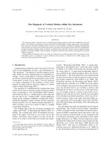
FIG. 1. Schematic view of a thermal. On the right panel, notations for the discretized scheme are presented: F k11/2 is the vertical mass flux per unit area at the interface between layer k and k 1 1; E k is the mass flux of air entering the thermal and D k is the detrainment for layer k (see appendix A for details).

frictionless, the vertical velocity inside the plume, in absence of phase change of water, is given by dw ]w u 2 u ML 5w 5 g SL dt ]z u ML

(3)

(horizontal pressure differences between the plume and its environment are neglected). The air is uniformly accelerated in the ML until the level where the mean potential temperature u (z) exceeds uSL . This level will be retained for definition of z i . At this level, the square of the vertical velocity wmax obtained by vertically integrating Eq. (3) over the depth of the CBL is twice the convective available potential energy (CAPE) defined as CAPE 5

E

0

zi

u 2 u ML g SL dz. u ML

0

zt

g

u SL 2 u dz 5 0. u

(5)

The integral corresponds to the shaded area on the lefthand side of Fig. 1 and the CAPE to that part of the integral below z i . After reaching z t , air parcels coming from the plume are heavier than the environment and should sink again. This will not be considered here. What is required for transport computations is not the vertical velocity but rather the mass flux per unit area, f 5 arw, where a is the fraction of the horizontal surface covered by ascending plumes and r is the air density. As a first step, we assume that f is constant within the ML (no detrainment). In order to determine this constant value, it is necessary to invoke the geometry of the thermal cell.

1 ]ps ]y 52 , ]y r s ]y

y

(6)

where p s is the surface pressure. Integrated over the width of a single cell, we obtain that the maximum horizontal velocity y max is given by 2 y max .

(4)

Above z i , w is still positive (overshooting) but decreases to finally vanish at the height z t (top), where

E

Let us consider a 2D configuration (roll) with an invariant horizontal direction x. The air in the thermal is supplied by horizontal convergence in the SL. If friction and rotation effects are neglected, and if the cell is stationary, the equation for the horizontal acceleration in the SL reduces to

2 Dp , rs s

(7)

where D denotes the difference between the conditions within the plume and those within the environment. If we assume that the pressure is identical in the plume and environment at a certain level, for instance z i , the surface pressure is just ps 5 p(z i ) 1

E

zi

gr dz.

(8)

0

We obtain to first order 2 y max .

2 D rs

.2

E

0

E

zi

gr dz

(9)

0

zi

g

r u SL 2 u ML dz rs u ML

(10)

by assuming that D r/r . D u/u. Except for the coefficient r/r s , of order 1 to 0.5 in the CBL, the computation is exactly that of the maximum vertical velocity wmax at

1108


height z i . Although this presentation is far from the real situation, y max 5 wmax is used for the parameterization. In a 2D geometry, the vertical mass flux in the thermal must equal the horizontal convergence of air in the SL:

VOLUME 59

simple square root dependency is retained for reducing the width of the thermal below z i , considering l as a tunable parameter. c. Model equations

wmax l(z i )r(z i ) 5 y max z s r(z s /2),

(11)

where l(z) is the width of the plume at height z. In this simple view, the width of the thermal at the inversion is roughly the height of the SL. The fact that near-surface horizontal converging winds are of the order of magnitude of vertical winds further implies that the width of a cell L is comparable to its height z t . For L k z t , indeed, air coming from distance L of the plume would reach the boundary layer top before reaching the plume, thus creating a secondary updraft. This isotropy is generally observed in Rayleigh–Beńard laboratory experiments. In nature, the aspect ratio r 5 L/z t typically ranges from 1 to 10 according to glider pilots (see also Moeng and Sullivan 1994; Atkinson and Zhang 1996). We introduce r as a tunable parameter in our model and obtain the minimum fractional area at level z i as a(z i ) 5 l(z i )/(rz t ) resulting in f 5

r (z s /2)z sÏ2CAPE rz t

.

The presentation above was done for an idealized temperature profile. In the complete formulation, the thermal is still characterized by a vertical velocity (wˆ), a potential temperature (uˆ ) and the fraction of the horizontal surface covered by thermals (aˆ ). The updrafts mass flux per unit of horizontal area is ˆf 5 raˆ wˆ (r is assumed to be the same inside and outside the thermal). Let us note, I(z, z9) 5

b. Detrainment and the environment Assuming that the upward mass flux is a constant leads to an infinite value of a at the top of the plume where w vanishes. In practice, this means that the plume is no longer conserving mass and that air must be supplied back to the environment. For the parameterization, we assumed that, above the inversion layer, the width of the thermal decreases to zero at z t (in practice, we tested both a linear and a quadratic decrease as explained further). In addition, we assume that the thermal can also detrain below z i due to small-scale turbulent mixing. This effect is accounted for by a shedding factor based on classical scaling arguments. The depth of the boundary layer of a jet with constant velocity w moving in a steady environment should grow as Ïlz (see, for instance, Prandtl and Tietjens 1934, chapter IV). In this simple context, l 5 n g /w where n g is the gas eddy viscosity. For a typical vertical velocity of 1 m s 21 and an eddy diffusivity of 10 m 2 s 21 , l 5 10 m. As a first step, this

z9

g

z

u (z) 2 u (z0) dz0. u (z0)

(13)

For unstable air (if locally, ]u/]z , 0), the CAPE is I[z, hi(z)] with hi(z) 5 min{z9 such that z9 . z and u (z) 5 u (z9)}. We also define the top of the thermal z t as the maximum value of ht(z) with ht(z) 5 min{z9 such that z9 . z and I(z, z9) 5 0}. The vertical variation of ˆf depends on the rate of horizontal entrainment in the surface layer eˆ and on detrainment dˆ : ] fˆ 5 eˆ 2 dˆ . ]z

(12)

The above analysis has assumed a 2D geometry (roll) for which observations suggest values of r of about 2– 3 (LeMone 1973; Moeng and Sullivan 1994); r 5 2 was retained as a nominal value for the parameterization. In the 3D case of isolated thermal plumes, scaling would probably be somewhat different. So r is used as a tunable parameter. Note that wmax /y max could be introduced as an additional free parameter.

E

(14)

Following the preceding analysis [and Eq. (12)] eˆ is expressed as eˆ (z) 5

r (z)Ï2I[z, hi(z)] rz t

,

(15)

where ]u/]z . 0 and 0 elsewhere. Below z i , detrainment is prescribed as dˆ (z) 5

ˆ Ïlz ] rw . ]z rz t

1

2

(16)

Above z i , the width of the thermal is reduced as [(z t 2 z)/(z t 2 z i )] m . Since eˆ 5 0 there, the detrainment between z i and z t writes as dˆ (z) 5 2

[

1

2

] z 2z rw ˆ aˆ (z i ) t ]z zt 2 zi

m

]

.

(17)

In the cases presented below, m 5 1 and m 5 2 were tested. The inversion level z i is defined as the height were the potential temperature inside the thermal uˆ becomes smaller than the environment (overshoot). Stationary conservation equations inside the thermal can be written ] fˆ f ˆ 5 eˆfe 2 dˆ f ˆ ]z

(18)

] fˆ w ˆ uˆ 2 u e 5 2dˆ w ˆ 1 gr , ]z ue

(19)

15 MARCH 2002

HOURDIN ET AL.

where f is any scalar including potential temperature and the subscript e stands for mean variables in the environment, around the thermal. The f e is related to the value inside the thermal f ˆ and to the mean value f at a given level through

f 5 aˆ fˆ 1 (1 2 aˆ )f e .

(20)

Note that eˆ has no contribution to Eq. (19) since the air is assumed to be supplied to the thermal with a zero vertical velocity. For vertical transport of horizontal momentum, the simplest idea is to treat both horizontal components u and y of the horizontal wind v as passive scalars [Eq. (18)]. This approach was retained as a first step. In reality, depending on the organization of mesoscale structures (cells, rolls, etc.), the thermal may exchange momentum with the environment through horizontal pressure gradients. A naive view suggests that this interaction should tilt the thermal in the direction of the dominant wind in the mixed layer. In such a configuration, the thermal would deposit its momentum well below the inversion level. It is premature to introduce such an effect in the standard version of the parameterization. However, as a sensitivity test, we introduced a simple formulation based on the drag formulation used to compute balloon drift in the atmosphere. This drag scales as the product of the apparent cross section of the balloon times the square of the apparent wind. The diameter of an isolated thermal plume (3D view, simpler for that purpose) scales as LÏaˆ so that the cross section of the thermal for a layer of width dz is LdzÏaˆ . The drag must be divided by L 2 (drag per unit horizontal area) to finally write the equation for momentum transport as Ïaˆ ] fˆ vˆ 5 eˆve 2 dˆ vˆ 1 gr \ve 2 vˆ \(ve 2 vˆ). ]z L

(21)

Here, g is used as a free parameter for sensitivity tests. The total transport of a variable f can finally be computed as the sum of upward transport in the thermal and downward transport in the environment, corresponding to a compensatory mass flux 2fˆ, as

r w9f9 5 fˆ (fˆ 2 fe ).

(22)

If integrated as such, Eq. (18) may lead to unrealistic values of f e . For instance, consider the case of a scalar initially confined in the surface layer in a situation with well-developed thermals. Equation (18) would predict fˆ . 0 in the mixed layer, where f 5 0 so that f e , 0. This problem arises from the hypothesis of stationarity. A simple way to rectify this is to assimilate the environmental and mean values (f e 5 f ) in the above equations. This approximation, valid for aˆ K 1, is generally used in mass flux parameterizations of deep convection. It is probably less valid in our case where aˆ is typically of the order of a few to 30%. However, this approach was retained as a first step.

1109

The scheme finally depends on four parameters. Nominal value for the aspect ratio, r 5 2, was chosen to agree with observations and simulations of rolls; g 5 0 was chosen for the sake of simplicity. The parameters for shedding were chosen in order to obtain a satisfactory agreement with LES results presented in the next section. Although different combinations are possible, we retained l 5 20 m and n 5 2. Discretization of the equations above is detailed in appendix A. d. Local closure The parameterization presented above accounts for the transport by thermals only. Small-scale turbulence, especially important in the surface layer, must be accounted for with an additional parameterization. For this, the Mellor and Yamada (1974, M&Y hereafter) 2.5 parameterization based on a prognostic equation for the turbulent kinetic energy is used. The version presented by Ayotte et al. (1996) based on Yamada (1983) is retained. Details are given in appendix B. In the simulations presented below, the thermals mass flux model and the M&Y scheme are called sequentially. 3. Comparison with LES As a validation of the new parameterization, comparisons with results from LES are presented. In the past decade, a number of numerical studies of the convective boundary layer were conducted with LES (see, in particular, Ebert et al. 1989; Schumann and Moeng 1991; Moeng and Sullivan 1994). In those simulations, the dynamics are solved explicitly down to a scale of typically 20 to 200 m. At the mesh scale, the nonlinear interactions with subgrid scales is parameterized using closure relations. LES are particularly well adapted to the study of the convective boundary layer for which resolved large-scale motions are believed to play a dominant role. There are two important advantages in validating a parameterization against LES rather than observations. The first one is that the experimental conditions are precisely known and can easily be modified. The second one is easier access to specific diagnosis. The new parameterization is validated using the LES results published by Ayotte et al. (1996). In this study, a number of boundary layer parameterizations were evaluated by comparison with a series of LES conducted in neutral and convective conditions. a. Description of the LES For a full description of the LES results, one should refer to Ayotte et al. (1996). Only a brief description of the model and cases is given here. The LES code, originally developed by Moeng (1984), is pseudospectral in the horizontal and finite difference in the vertical. The flow is horizontally homogeneous with periodic

1110


boundary conditions in both horizontal directions. The subgrid-scale parameterization is based on a prognostic equation for the turbulent kinetic energy. The simulations are all conducted for a water and cloud-free atmosphere in unstable or neutral conditions with a prescribed surface heat flux w9u9 0 . Nine simulations—00WC, 05WC, 00SC, 03SC, 05SC, 24SC, 24F, 15B, 24B—were conducted. They essentially differ by the value of the surface heat flux (05SC, for instance, means that the surface heat flux is of 0.05 K m s 21 ) and by the shape of the initial potential temperature profile. The WC simulations correspond to weakly capped profiles with a rather weak inversion opposite to strongly capped (SC) cases. For all the simulations labeled either SC or WC, there is a geostrophic wind of 15 m s 21 along the x direction. The 24F simulation is a case of free convection with no geostrophic wind and a surface heat flux of 0.24 K m s 21 . Cases 15B and 24B correspond to ‘‘baroclinic’’ forcing with a constant geostrophic wind of 10 m s 21 in x and a meridional geostrophic wind increasing linearly with height from zero at the surface up to 20 m s 21 at an altitude of 2 km. All the simulations were initiated with small perturbations and run over a period of time corresponding to 5 t, where t is a characteristic timescale (the convective time scale for the cases with nonzero surface heat fluxes ranging typically from 500 to 1000 s). The end of this period is used as the initial time t 0 for 1D simulations. Both the LES and 1D models are then run on 10 additional t starting from the same mean fields at t 0 . Comparisons are made from t1 5 t 0 1 4t to t 2 5 t 0 1 10t. Two tracers B and C are included in the simulations in addition to dynamical variables. Both are initiated at t 0 with a discontinuity at the inversion level z i as follows: B 5 13.5, 5 3.0, C 5 0.0, 5 1.0,

0 , z # 1.01z i z . 1.01z i

(23)

0 , z # 1.01z i z . 1.01z i .

b. 1D experiments The time evolution of variables u, y , u, B, and C is computed from the parameterization of the boundary layer processes with source terms: ]f 1 ]r w9f9 5 Sf 2 . ]t r ]z

[S u 5 f (y 2 y g ) and S y 5 2 f (u 2 u g )] and zero for the other variables. For potential temperature and tracer C, boundary conditions consist in prescribing the surface flux (zero for C). For winds and scalar B, boundary conditions are handled following Ayotte et al. (1996) based on Monin– Obukhov similarity theory and Businger–Dyer relationships:

[1 [1

(25)

The source term S f is the geostrophic forcing for wind

2

] 1 2] 12

\v1 \ 1 z 1 z0 z 5 ln 2 Cm u* K z0 L

2

(26)

B1 2 Bs 1 z 1 z0 z 5 ln 2 Ch , B* K z0 L

(27)

where v1 and B1 are wind and concentration of scalar B in the first model layer, K 5 0.4 is the Von Karman constant, and L is the Monin–Obukhov length expressed as a function of friction velocity u* and surface heat flux w9u9 0 : L52

u*3 u 0 . K gw9u 90

(28)

The stability functions for momentum and scalars can be written as

[1

21 2 11x C 5 2 ln 1 , 2 2

1 1 x2 Cm 5 ln 2

11x 2

2

]

2 2 tan21 x 1

p 2

(29)

2

(30)

h

with x 5 (1 2 15z/L)1/4

(31)

C m 5 C h 5 25z/L

(32)

for z/L , 0 and for z/L $ 0. Within the atmosphere, the parameterized turbulent flux w9f9 takes the general form

(24)

Tracer C is only transported whereas a surface flux is introduced for tracer B. This flux is computed from the contrast between atmospheric concentration and a surface value B s 5 15 (arbitrary units).

VOLUME 59

r w9f9 5 2rK f

1 ]z 2 G 2 1 fˆ (fˆ 2 f), ]f

f

(33)

where G f is a countergradient term. Three boundary layer parameterizations are compared. • Thermals: K f is computed with M&Y scheme and G f 5 0 for all variables. • M&Y: same thing without thermals (fˆ 5 0). • The Holtslag and Boville (H&B) parameterization as presented by Ayotte et al. (1996). Here, ˆf 5 0; K f is prescribed as a function of height including nonlocal aspects. The countergradient term G is nonzero for u, B, and C. H&B and M&Y simulations are duplications of those

15 MARCH 2002

HOURDIN ET AL.

1111

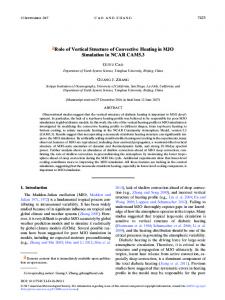
FIG. 2. Comparison of LES profiles with the results of the thermals model with nominal values of the parameters ( l 5 20, m 5 2, r 5 2, and g 5 0) for 4 cases (05WC, 05SC, 24SC, and 24F). For each case, the initial profile (dashed curve) and the average between times t1 and t 2 for the LES (thin solid curve) and for the parameterization (heavy solid curve) are shown. For the heat flux, there is no initial value. For the 24F case, winds are null.

presented by Ayotte et al. (1996). They have been rerun, as control simulations, in the same modeling environment as the new parameterization. The same vertical grid is used as for the LES, with a regular spacing of 10 or 20 m depending on the case. Depending on the case also, the time step varies from 15 to 100 s. c. Numerical results Figure 2 shows the vertical profiles of potential temperature, heat flux, scalars, and wind for representative

simulations, obtained with the thermals model and with the nominal values of parameters (l 5 20 m, n 5 2, r 5 2, and g 5 0). The initial profiles are shown as well as averaged values between t 0 1 4t and t 0 1 10t. The reasonable agreement of the parameterization with LES is in large part due to the forcing of these academic simulations with prescribed surface flux and capping inversion. The heat input is rapidly mixed below the capping inversion resulting in a homogeneous heating below the inversion. Figures 3 and 4 show the results for cases 05WC and 24SC for the H&B and M&Y parameterizations. The

1112


VOLUME 59

FIG. 3. Comparison of the results of the H&B parameterization with both LES and thermals model results for cases 05WC and 24SC.

H&B parameterization was shown to perform quite well in this context (Ayotte et al. 1996). It generally tends to slightly exaggerate the capping inversion. It overestimates the entrainment for case 05WC and slightly underestimates it for case 24SC. The M&Y scheme underestimates entrainment. The good agreement for heat fluxes is obtained for unstable temperature profiles, as expected for a local second-order closure. In order to quantify the intercomparison, Ayotte et al. (1996) proposed original diagnosis focusing on the transfer across the inversion layer. In particular, they

proposed to compute for a scalar quantity f (either u, B, or C) the quantity A1 5 2 5

1 t f 2 t1

1 t f 2 t1

E

E

H

[f (z, t f ) 2 f (z, t 0 )] dz

(34)

z i (t 0 )

tf

w9f9[z i (t 0 ), t] dt,

(35)

t0

where H is any height above the PBL top. A1 is a measurement of entrainment at the inversion layer. It is eas-

FIG. 4. Comparison of the results of the M&Y parameterization with both LES and thermals model results for cases 05WC and 24SC.

15 MARCH 2002

HOURDIN ET AL.

1113

ily computed with the first formula from the vertical profiles at t 0 and t f . Following Ayotte et al. (1996), we computed A1 using for final profiles the mean profiles between t1 and t 2 [t f 5 (t1 1 t 2 )/2]. For scalars B and C, A1 is exactly the area separating the dashed and solid curves above the discontinuity. Figure 5 shows for the 9 cases the A1 coefficient for the LES, the new parameterization with thermals in nominal configuration and the H&B and M&Y schemes. The M&Y parameterization tends to underestimate entrainment, which is not surprising for a local scheme. H&B overestimates entrainment for weakly capped cases and underestimates it for strongly capped cases. Both fail in predicting any significant entrainment for free convection. In the intercomparison by Ayotte et al. (1996), the same behavior was observed for all the tested schemes but one. Only a mixed layer approach was able to simulate entrainment of similar intensity for 24F and 24SC (this scheme was, however, significantly overestimating entrainment for all the cases). The agreement with LES is generally better for the thermals model for A1 coefficients as well as for air temperature close to the surface as illustrated in Fig. 6. d. Sensitivity to model parameters As mentioned above, the LES results have been used to select the nominal values of the model parameters. Figure 7 shows A1 parameters for u and B and for different values. The simulations are run for l 5 80 m, l 5 0 m, r 5 5, and m 5 1. Increasing l significantly decreases A1 for potential temperature for convective cases. Decreasing l to zero (neglecting shedding below the inversion layer) or using a less steep shedding above z i (m 5 1) results in a too strong overshoot for some cases. Note, however, that running the parameterization changing simultaneously l to 80 m and m to 1 produces results very similar to the nominal case. Changing the aspect ratio from 2 to 5 does not significantly affect the results. Finally, introducing a momentum exchange between the thermal and environment (tilted thermal, with g 5 0.5; see the discussion below) has only a weak impact on A1 coefficients. To end up with, note that, even far from the nominal values of the parameters, the thermals model keeps a good sensitivity to surface heat flux and initial profiles. For instance, for u, A1 for 24F is always just a little bit larger than for 24SC; A1 is also larger for 05SC than for 05WC. Note also that for tracer B the agreement is very good for all the cases (results are very similar for C). e. Inside thermals Figure 8 illustrates the structure of the thermal simulated with the nominal version of the parameterization as well as the decomposition of the heat flux in its smallscale part (dashed, right panel) and thermals (thin solid

FIG. 5. A1 parameters for potential temperature and scalars B and C for the 9 simulations. LES results are compared with the new parameterization (‘‘thermals’’) with nominal values of the parameters (l 5 20 m, m 5 2, r 5 2, and g 5 0) as well as with the H&B and M&Y schemes. For consistency with Ayotte et al. (1996) figures, A1 is divided by the mean value for the nine LES cases.

curve). Heat is first supplied from the surface to the SL by the M&Y scheme and then transported in the ML by thermals. In the mixed layer, thermals transport heat up the vertical gradient of potential temperature. Note that the situation is completely different when the M&Y is run alone (Fig. 4): there, the heat transport

1114


FIG. 6. Increment of air temperature in the first layer above the surface (value averaged between t1 and t 2 minus that at t 0 ).

VOLUME 59

FIG. 8. Structure of thermals for case 24SC. For the first panel, the thin (heavy) line corresponds to the fractional cover before (after) shedding. For w9u9 (last panel, heavy line) the decomposition into thermals (thin solid curve) and eddy diffusion (dashed curve) is shown.

by the M&Y scheme extends up to the inversion layer, thanks to a destabilized potential temperature profile. The fractional cover in the middle of the ML is of the order of 10%. Similar fractions are found for the other cases. Note that using r 5 5 produces accurate mean fields and fluxes but with a much smaller fractional cover (3%–5%). Those results are qualitatively in agreement with the analysis by Moeng and Sullivan (1994) on the same LES results (fractional cover of 10%–20% with an aspect ratio of 2–3 for intermediate cases). Aircraft measurements in similar conditions (Williams and Hacker 1993) lead to similar results. The values we find are, however, closer to the lower range of the observed or simulated ones. This must be related to the fact that only the buoyant air coming from the surface is considered as updraft in the parameterization. f. Second-order moments

FIG. 7. Normalized A1 parameter for potential temperature and scalar B are compared for LES, for the thermals model with nominal values of the parameters (l 5 20 m, m 5 2, r 5 2, and g 5 0) and for sensitivity experiments performed by changing one or two of the parameters. The ‘‘tilted’’ case corresponds to g 5 0.5 (see text for details). Heavy lines (LES and nominal) are already shown in Fig. 5.

The goal of a turbulent closure is to predict the effect of turbulence on mean fields, by in general analyzing part of the statistics of the turbulent fields. Whereas classical local closures favor a development at successive orders of the equations for turbulent fluctuations, the present approach focuses on the largest coherent structures. So, this parameterization is not particularly well suited for prediction of second or third moments of turbulent variables. However, the comparison with second-order moments for vertical wind and temperature (the only ones available to us) turned out to give some further insight into the physics of the convective boundary layer. The comparison is shown for cases 05WC and 24SC (Fig. 9). For the LES, the second order moments contain large eddies plus parameterized subgrid scales for the vertical wind and only the large eddies for temperature. For the parameterization, we show both the thermals contribution alone:

15 MARCH 2002

HOURDIN ET AL.

FIG. 9. Second-moment distribution of potential temperature and vertical wind for cases 05WC and 24SC for the LES (heavy curves) and nominal version of the new parameterization (thin curves). The dashed curves correspond to the contribution of the thermals model alone.

f92 5 aˆ (fˆ 2 f) 2 1 (1 2 aˆ )(fe 2 f) 2 5

aˆ (f ˆ 2 f) 2 , 1 2 aˆ

(36) (37)

and the total second-order moment computed as the sum of the thermals and local closure contributions (see appendix Ba for the prediction of second-order moments compatible with the M&Y model). In the surface layer, both wind and temperature fluctuations are well reproduced. The slight overestimation of u9 2 is probably due to the noninclusion of the parameterized component in the LES results. In the ML (for 0.1 # z/z i # 0.7), the prediction of u9 2 by the thermals model is also very close to LES results. On the other hand, the prediction of w9 2 is of the order of half the LES value. This can be understood as follows. In the ML, we essentially account for the largest structures based on the idealized view of an homogeneous thermal carrying air from the surface layer (see upper panels in Fig. 10). In reality, the air inside thermals (and outside to a lesser extent) is also turbulent on smaller scales. However, the temperature fluctuations associated with those small-scale fluctuations of w9 are small because u is quite uniform vertically, both inside and outside the thermal. With a Lagrangian view, a positive fluctuation of u is associated with an air parcel originating from the surface layer. In the inviscid limit,

1115

FIG. 10. Schematic view of horizontal tracs of w9 and u9 for the idealized thermal used for the parameterization (upper panels) and for a somewhat more realistic view including small-scale eddies (middle panels) are compared with composites derived form aircraft measurements (lower panels). The composites are taken from Williams and Hacker’s (1992) Fig. 5, and correspond to 0.2 # z/z i # 0.3. The full curve represents the mean structure of thermals. The dashed represents the associated variance coming from the various thermals sampled for the composite. In the composite analyses the thermals are superimposed on the same unit scale.

whether the trajectory of this parcel is a straight line or looks more like a random walk does not matter. This extended view of a turbulent thermal plume is illustrated in the middle panels of Fig. 10. Note that since the smallscale fluctuations of w9 are only marginally associated with fluctuations of u9, the two descriptions result in a comparable heat flux. The lower panels in Fig. 10 show an example of a composite view of real thermals in the ML (after Williams and Hacker 1992). In the analysis, composites are performed by isolating coherent plumes based on a threshold on u9. The selected regions are scaled horizontally to a unit length and averaged to give a mean view of the thermal. The positive fluctuations of u9 are of course associated with positive fluctuations of w9. Whereas the variance of the dispersion of the various thermals is comparable to the mean value inside the thermal for w9, it is only about one-third for u9, quite consistently with the idealized view given above. In fact, on raw measurements used for those composite analysis, the thermals are clearly visible for u9 but much more difficult to identify for w9 [see Williams and Hacker’s (1993) Fig. 13]. In the entrainment zone, the parameterization is clearly unable to give even a crude estimation of u9 2 and w9 2 . The processes involved in this region include overshooting (partly accounted for), sinking of overshooted air, Kelvin–Helmholtz and internal gravity waves. All those processes are accounted for crudely through irreversible mixing of detrained air with environment. For instance, the strong reduction of the mesh fraction as-

1116


VOLUME 59

TABLE 1. Overview of the meteorological conditions over Paris during the IOP 2 (8 and 9 Aug 1998). Day Wind direction (from) |U| (10 m) (m s21 ) /h¯ (max) (m) T 2m min (8C) T 2m min (UTC) T 2m max (8C) T 2m max (UTC)

8A98

9A98

E

S to E 1.8 2800 18.7 0500 35.0 1500

1.3 2300 17.5 0600 35.3 1600

convective situation over the Paris area, documented in the frame of the ESQUIF project are presented. These simulations are designed in a context closer to largescale meteorological or climate modeling (forcing by radiation, coarser vertical grid, etc.). a. The study case FIG. 11. Horizontal wind component u for the thermals model in its nominal configuration and with inclusion of an horizontal drag (g 5 0 and 0.5, respectively). The figures show for cases 05WC and 24SC, the initial profile, the mean profile as obtained with LES and with the parameterization as well as the value inside the thermal, uˆ.

sociated with overshooting above z i hides the fact that the air can overshoot and then come back being finally mixed by turbulence below its level of maximum excursion. Accounting properly for those motions could produce a similar heating with a very different value of u9 2 . The same thing can be said for gravity waves generated by overshooting that are not expected to exchange heat with the mean flow in the linear limit. The fact that the temperature fluctuations are still very large at z/z i 5 1.5 in the LES, at an altitude where w9u9 5 0, emphasizes the fact that only part of the turbulent fluctuations are involved in heat processes. g. Momentum transport Figure 11 compares the horizontal momentum for the nominal configuration and for the parameterization with drag (g 5 0.5). In the standard parameterization, the horizontal momentum has a constant value inside the thermal above the surface layer. When drag is introduced, the horizontal wind inside the thermal converges to the value in the environment thus producing a tilt of the thermal. This kind of refinement could be introduced easily in the parameterization but would require a detailed analysis of observations or LES, and should probably strongly depend on the geometry of mesoscale structures. However, the impact on heat and scalar fluxes and even on momentum is weak. 4. ESQUIF IOP 2 simulation To further illustrate the behavior of the new parameterization, one-dimensional numerical simulations of a

ESQUIF is a project dedicated to the study and modeling of air quality in the Paris area (Menut et al. 2000). The campaign was designed as a series of intensive observation periods (IOPs) each of duration 1 to 5 days. Among them was IOP 2, which consisted of a very hot and convective situation with rather weak winds and no clouds, thus an ideal situation for testing parameterizations of the CBL. The IOP 2 occurred from 7 to 11 August 1998, the major pollution event of the summer of 1998 in the Paris area. During this period, strong surface pollutant concentrations were observed on 8 and 9 August 1998 (hereafter called 8A98 and 9A98). As shown in Table 1, this period corresponds to a low wind, high temperatures, and a cloud-free period corresponding to typical conditions for a well-developed CBL. For model validation, two sets of observations are used: • Measurements of temperature, relative humidity, and pressure at 2 m above ground level (AGL) recorded hourly at the stations of the Me´teó-France meteorological surface network (Mesonet) spread over a large area around Paris. • Soundings performed by Me´teó-France in Trappes (25 km southwest of Paris). Temperature, relative humidity, pressure, and wind speed and direction soundings are routinely available at 0000 and 1200 UTC. During IOP 2, additional soundings were obtained every 3 hours. Figure 12 illustrates the evolution of the boundary layer (BL) structure during IOP 2. The BL depth is superimposed on soundings of virtual potential temperature. It is computed using a threshold for the bulk Richardson number, R ib . 0.21, with R ib (z) 5

g(z 2 z 1 ) [u (z) 2 u (z 1 )] u (z) u(z) 2 1 y (z) 2

(38)

15 MARCH 2002

HOURDIN ET AL.

FIG. 12. Virtual potential temperature profiles recorded at Trappes for the 8 and 9 Aug 1998 and corresponding boundary layer depth (dots; see text for details). Profiles are time shifted, following the launching date: the time reference corresponds to the surface point on each profile and the relation between time and temperature is 2.75 K h 21 for each of them.

(Menut et al. 1999). For soundings, we consider the altitude reference z1 as the first vertical point available on the profile (from 0 to 50 m, as all profiles have different recorded altitudes). As previously explained, days 8A98 and 9A98 correspond to typical conditions of a well-developed CBL. At the beginning of 8A98, the nocturnal boundary layer appears at 300 m surmounted by a thin residual inversion layer (around 2300 m). At the sunrise, convective effects increased rapidly. The residual layer was mixed out around 1000 UTC. The second synoptic inversion was eroded at 1200 UTC and the top of the BL reached 2300 m. The situation was similar during 9A98. A large thermal inversion was observed above 2800 m in the afternoon. b. The model The ESQUIF IOP 2 results are obtained using the LMDZ general circulation model (GCM) in its onedimensional configuration. LMDZ is a Labroatoire de Me´teórologie Dynamique gridpoint global primitive equation model with zooming capability (Z). It is used currently for climate studies (Krinner et al. 2000) and simulation of the atmospheric transport of trace species (Hourdin and Armengaud 1999; Hourdin and Issartel 2000). LMDZ is also the atmospheric component of a complete climate model including biosphere, ocean, and chemistry, under development at Institut Pierre Simon Laplace, in Paris. Coupled to large-scale atmospheric dynamics, the current version of LMDZ includes the radiation scheme of European Centre for Medium-Range Weather Forecasts: the solar part is a refined version of the scheme developed by Fouquart and Bonnel (1980) and the thermal infrared part is due to Morcrette et al. (1986). The surface model includes a 11-layer conduction

1117

scheme developed for Mars (Hourdin et al. 1993). The soil is assumed to be homogeneous with constant conduction j and specific heat per unit volume C. The conduction flux below the surface writes F c 5 2I]T/]z9 and the conduction equation below the surface ]T/]t 5 ] 2 T/]z9 2 . I 5 ÏjC is called thermal inertia and z9 is a pseudo depth defined as z9 5 zÏC/j. Following Laval et al. (1981), the surface evaporation is computed as E 5 1.35bru 2 [q s (T s ) 2 q] where q is * the specific humidity in the first atmospheric layer and q s (T s ) is the saturated specific humidity at the soil temperature. Here, the aridity coefficient b was used as a tunable parameter. Concerning the boundary layer, the new parameterization replaces the old local-K/countergradient approach as well as a convective adjustment [see Laval et al. (1981) for a description of the old boundary layer scheme]. We also ran numerical experiments with the M&Y scheme with no thermals and with the H&B scheme. The surface drag is computed according to Louis (1979). In the 1D simulations presented here, a vertical grid with 40 layers is used. The vertical discretization of the boundary layer is chosen to be similar to state-of-theart GCMs. The first layer is centered at about 40 m above the surface and layer 15 is at about 4.4 km with a vertical resolution of about 500 m between 1.5 and 3.5 km. c. Model parameters and forcing Simulations were conducted from 7A98 to 9A98 with meteorological fields initiated according to Trappes soundings of 6A98 at 2330 UTC. 7A98, which did not show a well-developed CBL, is considered as a ‘‘spinup’’ period for the physical parameterizations. Meteorological fields are once again initiated with the soundings of 8A98 at 530 UTC. Results are presented for 8A98 and 9A98. The surface albedo was fixed at 0.19, the surface roughness length at 0.4 m, a typical suburban value. The surface thermal inertia I was tuned to 3000 J m 22 s 21/2 K 21 , a typical value for dry continental surfaces, so as to reproduce the amplitude of the diurnal oscillation of the surface temperature. The initial temperature was fixed to 292 K in the 11 layers of the soil model and at the surface. b was tuned to 0.08 to have a drift of the near-surface humidity on the 3-day simulation comparable with observations. Although winds were moderate to weak during that period, a large-scale forcing is required. For water vapor, and since IOP 2 is cloud free, the model specific humidity is only affected by the boundary layer parameterization. In the free atmosphere, a systematic drying is visible in the soundings during 8A98 probably due to the advection of continental air from south. In order to keep the forcing as simple as possible, we rather specify it as a downward advection:

1118


FIG. 13. Comparison between mesonet (gray, 2 m AGL), soundings (dots) and model (curves) time series of temperature (K, upper panel) and specific humidity (g kg 21 , middle panel) for 8 and 9 Aug 1998. Soundings values are averaged over the depth of the first model layer. The bottom panel shows, with same conventions, the height of the boundary layer estimated using a threshold on the bulk Richardson number [Eq. (38)].

]q ]q 5 2w , ]t ]p

(39)

with w 5 w 0 3 sin(2pp/p s ). The w 0 was tuned to 0.6 Pa s 21 (corresponding to about 1 cm s 21 in the midtroposphere) during 8A98 and zero for 9A98, so as to reproduce the drying observed above the CBL. In principle, the derivation is not as straightforward for temperature since it is also affected by radiation. However, since the radiative computation is probably rather accurate in IOP 2 cloud-free conditions, the same approach was used. Results showed that some additional heating was required in order to obtain the observed temperatures above the boundary layer. Finally, the same form was used as for specific humidity, but with w 0 5 0.3 Pa s 21 during 8A98 and zero for 9A98. In the simulations presented here, horizontal wind components u and y are directly forced with values linearly interpolated in time from two consecutive soundings. For ESQUIF IOP 2 simulations, a time step of 3 min was used.

VOLUME 59

FIG. 14. Observed and simulated virtual potential temperature and specific humidity for 9A98.

d. Results We first present comparisons of the new parameterization in its nominal configuration (l 5 20 m, n 5 2, r 5 2, and g 5 0) with both observations and M&Y and H&B parameterizations. Figure 13 compares temperature and specific humidity simulated in the first model layer with the Trappes soundings values at the same level and with the 2-m measurements by the Me´teó-France network. Note that the model forcing was derived so as to reproduce satisfactorily near-surface humidity and temperature corresponding to Trappes soundings values averaged over the depth of the first atmospheric layer (dots in Fig. 13). The station measurements, being closer to the surface, give an idea of the stability in the surface layer and of the subgrid-scale fluctuations of meteorological fields in this area. Figure 14 shows a comparison between Trappes soundings and model results for virtual potential temperature u y (K) and specific humidity q (g kg 21 ). The two upper figures correspond to 0530 UTC 9 August 1998 and the two lower to 1730 UTC on the same day. For the 0530 UTC soundings, profiles show two major inversion layers. The lower one appears to be the nocturnal boundary layer, with a strong vertical gradient around 500 m AGL. The nocturnal boundary layer is quite well caught by the three parameterizations. In fact,

15 MARCH 2002

HOURDIN ET AL.

FIG. 15. Sensitivity to model parameters: potential temperature and specific humidity at 1730 UTC for 9A98, obtained by varying values of the thermals model parameters.

the M&Y parameterization was modified following Holtslag et al. (1990) in order to handle correctly those very stable conditions as explained in appendix Bc. The residual inversion layer (ø2200 m) is better simulated with thermals due to a better simulation of the CBL during 8A98. Above this residual layer, profiles of temperature and humidity are essentially determined by the large-scale forcing we use. The 1730 UTC profiles are characteristic of the convective processes occurring in early afternoon. The thermals parameterization shows a much better agreement with soundings, with a boundary layer height above 2500 m whereas the H&B and M&Y schemes find it around 2000 m. The overestimate of q above 2700 m is due to the specification of the large-scale forcing. The same sensitivity experiments as for the LES (l 5 80 m, l 5 0 m, m 5 1, and r 5 5) show a much smaller dispersion of the results (Fig. 15). Note in particular that the detail of the detrainment above the inversion layer is less important because of the larger depth of the model layer in the present case. The inversion and top of the PBL are generally separated by one layer only. 5. Concluding remarks We have shown that a simple parameterization of the CBL, based on an idealized mass flux representation of thermals, is able to well reproduce the main characteristics of the CBL dynamics and to transport heat upward in a slightly stable atmosphere without any need for ad hoc countergradient correction. The scheme seems to behave even somewhat better than classical parameterizations such as H&B and M&Y. In particular, the thermals parameterization reproduces very well the sensitivity of entrainment to the surface heat flux and initial profile. In addition, the parameterization is able to sim-

1119

ulate correctly not only heat fluxes but also temperature variances by accounting for half of the variance of the vertical wind only. This is fully consistent with the current picture of CBL transport being dominated by largescale coherent structures. It is also consistent with the observation that horizontal tracks in the ML exhibit more small-scale fluctuations for vertical wind than for temperature or humidity. The thermals model has some similarities with the scheme developed by Pleim and Chang (1992; see also Alapaty et al. 1997). In, their Asymmetrical Convective Model, based on a transilient matrix, upward transport by convective plumes is accounted for by mixing air directly from the first model layer to all other layers in the CBL. On that point, the thermals parameterization is quite similar except that the air is not taken in the first model layer only. For downward transport, the two parameterizations are also equivalent in that the transport is local. However, the two schemes strongly differ in the way they compute transport coefficients. Pleim and Chang (1992) compute the upward mixing coefficient as a function of surface heat flux, decreasing from the surface up to the inversion layer. This computation is similar to that of the vertical mixing coefficient and countergradient term proposed by Troen and Mahrt (1986) and used in the H&B scheme. Both schemes are also derived so as to account for turbulent and mesoscale transport from the surface up to the inversion layer. In the thermals parameterization on the other hand, the computation of velocities and fractional cover of thermals is based on the buoyancy of the air inside the plume. The mass flux computation is not directly related to surface fluxes. Instead, the closure is done in terms of CAPE [Eq. (12)]. Heat is first transferred to the SL by small-scale turbulence and then transported in the ML by parameterized mesoscale thermals. The computation of mass fluxes also allows a significant overshoot. The thermals model depends on 4 parameters: r was fixed to 2 in the range of observed or simulated values for roll configurations (LeMone 1973; Moeng and Sullivan 1994); g was fixed to 0 for the sake of simplicity; and parameters for the shedding (l 5 20 and n 5 2) were tuned using Ayotte et al. (1996) LES results. However, the parameterization is only weakly sensitive to these values. In particular, the A1 coefficient for scalar B was very marginally affected in sensitivity tests. The sensitivity is even much less when the model is run in a GCM-like configuration. Generally speaking, the sensitivity is weaker than the discrepancy between the different parameterizations. The parameterization may be tuned, refined or modified in several ways, particularly the shedding and geometry of the plumes. Good agreement can be obtained for l of the order of 10–100 m. Even for l 5 0, the behavior is still satisfactory, which could suggest that shedding has a rather weak influence on transport processes below the inversion layer (for l 5 0, detrainment

1120


occurs above z i only). Not only the width of the thermal plume but also its speed and mean potential temperature can be affected by small-scale turbulent mixing. Recently, Van Dop (2000) analyzed LES of the CBL in terms of the distributions of vertical velocities and potential temperature. They proposed a parameterization based on probability distribution functions with similar considerations on the asymmetry between concentrated thermal plumes and slow downward compensation. However, they assumed a significant impact of mixing on the strength of the thermal plumes. The real importance of shedding and mixing of thermal plumes in the ML thus remains an open question that should be addressed with different diagnostics of LES results as well as with in situ measurements aboard aircraft equipped with instruments with fast response times (see, for instance, Cruette et al. 2000). The composite approach by Williams and Hacker (1992, 1993) seems to be particularly well suited to make the link between observations, LES and parameterization of thermals. Similar techniques, based on conditional sampling, have already been applied to LES to try to separate updrafts and downdrafts (e.g., Schumann and Moeng 1991). However, the sampling condition favored in this particular study was the sign of the vertical wind, which is not selective enough to make a link with the parameterization proposed here. Only one analysis was completed with a positive threshold (and negative for downdrafts) on the vertical velocity to compare with observations of the marine boundary layer by Greenhut and Khalsa (1982). Qualitatively, the structure of the updraft seems to agree quite well with that obtained from the parameterization with a fractional cover of the order of 15%. The aspect ratio does not significantly affect the boundary layer transport. However, the same transport is obtained for quite different values of the fractional cover aˆ in the range of 3%–5% for r 5 5 and 20%– 30% for r 5 1 in the mixed layer. For the nominal case, simulated fractions are in the range of observations (Williams and Hacker 1993) and LES results (Moeng and Sullivan 1994). The description of the thermals geometry could be refined further, for instance, by taking different values of r for shear- or buoyancy-dominated thermals. Another important improvement may concern the computation of the potential temperature of the air supplied to the thermal in the surface layer. This temperature may be quite different (probably somewhat larger) from the mean temperature of the GCM mesh due to horizontal fluctuations related, for instance, to variations in surface albedo, presence of cities, variations in surface orography, or presence of lakes or rivers. The parameterization is currently being tested in the 3D GCM. The 3D application opens a series of questions concerning the interaction of the CBL dynamics with other processes. For instance, the fraction of wet air coming from the surface could be used for specification of cloud cover or horizontal variance of specific hu-

VOLUME 59

midity within a GCM mesh. Latent heat release could also be added to the CAPE computation in case of saturated plumes. However, it would be unwise to attempt extension to the case of fully developed deep convection, which operates on completely different scales with different physical processes involved. So the present parameterization should probably be limited in some way to the case of cumulus topped CBLs with moderate role of condensation processes. Most GCMs distinguish between boundary layer processes, treated with parameterizations inherited from similarity theory in which nonlocal aspects are included, and parameterizations which account for both shallow and deep convection. We alternatively suggest a distinction based in terms of scales in which small-scale transport (for which similarity theory is relevant), mesoscale transport (dry thermals, cloud streets, rolls, open or closed cells, shallow convection), and deep convective transport are each treated separately. Other uses of the parameterization are envisaged. One motivation for developing this thermals model was the atmosphere of Mars, for which a GCM has been developed at Laboratoire de Me´teórologie Dynamique (Hourdin et al. 1993). Mars, with dry atmosphere and no oceans, is indeed a very interesting case of global dry CBL. This parameterization could also probably be adapted with minor changes for modeling of deep water formations in the ocean. Acknowledgments. We are most grateful to Dr. Ayotte for having kindly provided the LES results and the sources of some of the codes he used, including the version of the Holtslag and Boville parameterization used in this study. We also want to thank very much Alain Lahellec and Jean-Yves Grandpeix. By their numerous discussions and knowledge of the boundary layer dynamics and mass flux parameterizations of deep convection, they significantly contributed to this work. We also want to thank Denise Cruette for her enlighting descriptions of the thermals reality and Robert Haberle for his help on the revised manuscript. This study was funded by Centre National de la Recherche Scientifique. APPENDIX A Discrete Formulation of the Thermals Mass Flux Model a. Thermals For the development presented below, GCM variables such as temperature or humidity are assumed to represent the mean value within a layer (finite-volume approach). For notations, integer indices for GCM variables and half indices for interfaces between two layers are used (see right-hand side of Fig. 1). The numerical scheme used to describe the mass fluxes is the following:

15 MARCH 2002

1) First the unstable layers k for which u k . u k11 , which together constitute the surface layer are detected. For each of them, the level l k is computed so that u lk # u k , u lk11 (inversion layer as seen by the air coming from layer k). We further integrate vertically from layer k:

O ug (u 2 u )(z

aˆ l11/2 5 aˆ li

k

j5k11

j

j11/2

2 z j21/2 ).

Ek 5

aˆ l11/2 (c) Fˆ l11/2 5 Fˆ l11/2 , (c) aˆ l11/2

(A1)

j

Following Eq. (12), the mass flux of air entering the thermal in layer k is defined as

r k (z k11/2 2 z k21/2 )Ï2Ik,Ik rz t

.

O Eˆ uˆ k5l

k

uˆ l 5

k

k51

, (c) Fˆ l11/2

(A3)

O Eˆ .

(A4)

ˆ k 1 Fˆ k11/2 . Eˆ k 1 Fˆ k21/2 5 D

k

(A10)

For any scalar f, we first compute the stationary solution inside the thermal following Eq. (18) discretized using an upstream scheme as ˆ kf Eˆ k f k 1 Fˆ k21/2 f ˆ k21 5 D ˆ k 1 Fˆ k11/2 f ˆ k.

k5l

(A9)

b. Convective transport

with (c) Fˆ l11/2 5

(A8)

and the detrainment mass flux D k is finally given by continuity

(A2)

Note that E k /(z k11/2 2 z k21/2 ) is the estimate of eˆ. The height of the thermal l t is defined as the highest l for which one of the I k,l21 is strictly positive. 2) We first integrate Eqs. (14) and (18) for uˆ assuming a conservative thermal (dˆ 5 0). The potential temperature is computed as

[ ]

n

lt 2 l . lt 2 li

Once this fraction is computed, mass fluxes are modified as

j5l

Ik,l 5

1121

HOURDIN ET AL.

(A11)

The tracer time evolution in a layer k is given by the divergence of the vertical flux

k51

We can further compute the vertical velocity in the thermal

1

(c) 1 2 1 Fˆ l21/2 w ˆ l11/2 5 w ˆ l21/2 (c) ˆ 2 2 Fl11/2

rk

2

2

O g uˆ 2u u (z

]f k 5 Fˆ k21/2 f ˆ k21 2 Fˆ k11/2 f ˆ k 1 Fˆ k11/2 f k11 ]t 2 Fˆ k21/2 f k .

l

1

k

k51

k

k11/2

2 z k21/2 ).

APPENDIX B

(A5)

k

In this discretized form of Eq. (19), the coefficient (c) (c) Fˆ l21/2 /Fˆ l11/2 accounts for the fact that only the air coming from the layer below in the thermal was at velocity wˆ l21/2 whereas the air coming from the environment at layer l must be accelerated vertically from zero. The inversion level l i is further defined as the value of k for which wˆ k11/2 is maximum. The fraction of the area corresponding to a conservative (no detrainment) thermal is then just (c) Fˆ l11/2 (c) aˆ l11/2 5 . (A6) w ˆ l11/2 r l11/2 3) Detrainment is computed from the surface up to the inversion level l i by reducing the fraction aˆ as

1

aˆ l11/2 5 max aˆ Above l i ,

(A12)

(c) l11/2

2

Ïlz l11/2 rz i

2

,0 .

Mellor and Yamada Parameterization The M&Y scheme is used both in the new parameterization, in order to account for small-scale mixing, and alone, for comparisons.

a. Equations In the version used, we follow Yamada (1983) and Ayotte et al. (1996). The eddy diffusivity is written K f 5 lqS f . Different stability functions are used for momentum, S m , potential temperature, S h 5 vS m and other scalars, S f 5 0.2. The mixing length l is computed as l 5 l0

(A7) with

Kz , K z 1 l0

(B1)

1122


E E

`

l 0 5 0.2

l w92 5 c 8 q 2 1 c 9 K h N 2 , q

zq dz

0

,

`

(B2)

q dz

0

Sm 5 1.96

(0.1912 2 Ri f )(0.2341 2 Ri f ) , (1 2 Ri f )(0.2231 2 Ri f )

Sm 5 0.085,

v 5 1.1318

0.2231 2 Ri f , 0.2341 2 Ri f

v 5 1.12,

(B3)

Ri f $ 0.16,

(B4)

Ri f , 0.16,

(B5)

Ri f $ 0.16.

(B6)

with c 8 5 0.24 and c 9 5 5.17. The fist term is dominant in the estimations presented here and corresponds to an estimation of w9 2 slightly smaller than equipartition of kinetic energy (c 8 5 1/3).

The prognostic equation for the turbulent kinetic energy on the one hand and the vertical diffusion of u, y , and scalars on the other are treated sequentially. The straightforward treatment of Eq. (B9), consisting in taking the right-hand side as a constant over the time step, converges only for very small time steps (of the order of a few seconds for the LES simulations). Instead, we rewrite this equation (without vertical diffusion) 1 ]q 2 5 q3x 2 ]t

Ri f 5 0.6588[Ri 1 0.1776 2 ÏRi 2 0.3221Ri 1 0.03156 ], 2

Ri , Ri c

(B7)

Ri $ Ri c ,

(B8)

where Ri fc 5 0.191 and Ri c 5 0.195 are critical Richardson numbers. The time evolution of q is computed from a prognostic equation for the kinetic energy,

[

]

1 ]q 2 q3 ] ]q 2 /2 5 Km M 2 2 Kh N 2 2 1 lqSq , 2 ]t lB1 ]z ]z

(B9)

as the sum of a source proportional to the wind shear M 2 5 \]v/]z\ 2 , an inhibition due to stratification with N 2 5 (g/u)(]u/]z), a dissipation in q 3 and vertical diffusion, with B1 5 16.6 and S q 5 0.2. Following Abdella and McFarlane (1997), secondorder moments for vertical wind and temperature are diagnosed based on the evolution equations ]w92 2 ]p9 ]w93 g 2 5 2 w9 2 1 2 w9u 9 2 e ]t r ]z ]z u 3

(B10)

]u 92 ]w9u 92 ]u 52 2 2w9u 9 2 2e u . ]t ]z ]z

(B11)

For temperature, neglecting third-order terms, assuming stationarity, retaining for the dissipation term e u 5 qu9 2 /(c12 l) with c12 5 9.1 (Abdella and McFarlane 1997) and replacing w9u9 by K h]u /]z leads to

u 92 5 c12 l 2 Sh

1 2. ]u ]z

(B13)

b. Numerics

Ri f , 0.16,

The flux Richardson number Ri f is derived from the gradient Richardson number Ri as

Ri f 5 Ri f c ,

VOLUME 59

2

(B12)

The treatment for vertical wind is less straightforward. We directly used Eq. (51) from Abdella and McFarlane (1997) but neglected third-order terms:

or

12

(B14)

] 1 5 2x, ]t q

(B15)

lSm 2 1 M (1 2 Ri f ) 2 . 2 q lB1

(B16)

with

x5

If x is assumed to be constant during the time step, the solution of Eq. (B15) is q (t1dt) 5

q (t) . 1 2 x (t) q (t) dt

(B17)

This solution is retained when x $ 0. When x , 0, we rather use q (t1dt) 5 q (t) (1 1 x (t) q (t) dt).

(B18)

This numerical formulation leads to numerical results almost indistinguishable from the first formulation but with time steps of typically 15 s to a few minutes for the simulations presented here. The vertical diffusion of q 2 is applied afterward. c. Special treatment for very stable conditions The formulation above leads to an unrealistically thin nocturnal boundary layer (NBL) in the ESQUIF simulations. In the H&B parameterization, such very stable conditions receive a special treatment (Holtslag et al. 1990). The PBL height must be greater than a minimum mechanical mixing depth prescribed as h 5 cu*/ f , (B19) where f is the Coriolis factor and c 5 0.07. In these conditions, the H&B scheme predicts a mixing coefficient

15 MARCH 2002

HOURDIN ET AL.

1

2

1

2

2

z , (B20) h where w m is a turbulent velocity scale for momentum asymptotic to u* at the surface. In our implementation of the M&Y scheme, we impose that, for stable conditions, K m remains larger than K m 5 K wm z 1 2

2

z . (B21) h If this threshold is reached, we take for the next time step q 5 Kmin /(KzS m ). This special treatment was essential to obtain a good agreement with soundings in the NBL, but it does not affect the results when thermals are active. It was not included for the comparison with LES since we wanted to favor convergence with Ayotte et al. (1996) results. It has a slight effect on cases 00SC and 00WC only. K min 5 K u*z 1 2

REFERENCES Abdella, K., and N. McFarlane, 1997: A new second-order turbulence closure scheme for the planetary boundary layer. J. Atmos. Sci., 54, 1850–1867. Alapaty, K., J. E. Pleim, S. Raman, D. S. Niyogi, and D. W. Byun, 1997: Simulation of atmospheric boundary layer processes using local- and nonlocal-closure schemes. J. Appl. Meteor., 36, 214– 233. Arakawa, A., and W. H. Schubert, 1974: Interaction of a cumulus cloud ensemble with the large-scale environment, Part I. J. Atmos. Sci., 31, 674–701. Atkinson, B. W., and J. W. Zhang, 1996: Mesoscale shallow convection in the atmosphere. Rev. Geophys., 34, 403–431. Ayotte, K. W., and Coauthors, 1996: An evaluation of neutral and convective planetary boundary-layer parameterizations relative to large eddy simulations. Bound.-Layer Meteor., 79, 131–175. Bougeault, P., and P. Lacarre`re, 1989: Parameterization of orography induced-turbulence in a mesobeta-scale model. Mon. Wea. Rev., 117, 1872–1890. Cruette, D., A. Marillier, J.-L. Dufresne, J.-Y. Granpeix, P. Nacass, and H. Bellec, 2000: Fast temperature and true airspeed measurements with the airborne ultrasonic anemometer-thermometer (AUSAT). J. Atmos. Oceanic Technol., 17, 1020–1039. Deardorff, J. W., 1972: Theoretical expression for the countergradient vertical heat flux. J. Geophys. Res., 77, 5900–5904. Ebert, E. E., U. Schumann, and R. B. Stull, 1989: Nonlocal turbulent mixing in the convective boundary layer evaluated from largeeddy simulation. J. Atmos. Sci., 46, 2178–2207. Emanuel, K. A., 1991: A scheme for representing cumulus convection in large-scale models. J. Atmos. Sci., 48, 2313–2335. Fouquart, Y., and B. Bonnel, 1980: Computations of solar heating of the Earth’s atmosphere: A new parameterization. Contrib. Atmos. Phys., 53, 35–62. Greenhut, G. K., and S. J. S. Khalsa, 1982: Updraft and downdraft events in the atmospheric boundary layer over the equatorial Pacific Ocean. J. Atmos. Sci., 39, 1803–1818. Holtslag, A. A. M., and B. A. Boville, 1993: Local versus nonlocal boundary-layer diffusion in a global climate model. J. Climate, 6, 1825–1842. ——, E. DeBruijn, and H. Pan, 1990: A high resolution air mass transformation model for short-range weather forecasting. Mon. Wea. Rev., 118, 1561–1575. Hourdin, F., and A. Armengaud, 1999: The use of finite-volume methods for atmospheric advection of trace species. Part I: Test of various formulations in a general circulation model. Mon. Wea. Rev., 127, 822–837.

1123

——, and J.-P. Issartel, 2000: Sub-surface nuclear tests monitoring through the CTBT xenon network. Geophys. Res. Lett., 27, 2245–2248. ——, P. Le Van, F. Forget, and O. Talagrand, 1993: Meteorological variability and the annual surface pressure cycle on Mars. J. Atmos. Sci., 50, 3625–3640. Krinner, G., D. Raynaud, C. Doutriaux, and H. Dang, 2000: Simulations of the Last Glacial Maximum ice sheet surface climate: Implications for the interpretation of ice core air content. J. Geophys. Res., 105, 2059–2070. Laval, K., R. Sadourny, and Y. Serafini, 1981: Land surface processes in a simplified general circulation model. Geophys. Astrophys. Fluid Dyn., 17, 129–150. LeMone, M. A., 1973: The structure and dynamics of horizontal roll vorticies in the planetary boundary layer. J. Atmos. Sci., 30, 1077–1091. Louis, J.-F., 1979: A parametric model of vertical eddy fluxes in the atmosphere. Bound.-Layer Meteor., 17, 187–202. Mellor, G. L., and T. Yamada, 1974: A hierarchy of turbulence closure models for planetary boundary layers. J. Atmos. Sci., 31, 1791– 1806. Menut, L., C. Flamant, J. Pelon, and P. H. Flamant, 1999: Urban boundary layer height determination from lidar measurements over the Paris area. Appl. Opt., 38, 945–954. ——, and Coauthors, 2000: Atmospheric pollution over the Paris area: The ESQUIF project. Ann. Geophys., 18, 1467–1481. Moeng, C., 1984: A large-eddy-simulation model for the study of planetary boundary-layer turbulence. J. Atmos. Sci., 41, 2052– 2062. ——, and P. P. Sullivan, 1994: A comparison of shear- and buoyancydriven planetary boundary layer flows. J. Atmos. Sci., 51, 999– 1022. Morcrette, J. J., L. Smith, and Y. Fouquart, 1986: Pressure and temperature dependence of the absorption in long-wave radiation parameterizations. Contrib. Atmos. Phys., 59, 455–469. Pielke, R. A., and M. Uliasz, 1998: Use of meteorological models as input to regional and mesoscale air quality models—Limitations and strengths. Atmos. Environ., 32, 1455–1466. Pleim, J. E., and J. S. Chang, 1992: A non-local closure model for vertical mixing in the convective boundary layer. Atmos. Environ., 26A, 965–981. ——, and A. Xiu, 1995: Development and testing of a surface flux and planetary boundary layer model for application in mesoscale models. J. Appl. Meteor., 34, 16–32. Prandtl, L., and O. G. Tietjens, 1934: Applied Hydro- and Aeromechanics. Engineering Society Monogr., Dover, 311 pp. Raymond, D. J., and A. M. Blyth, 1986: A stochastic model for nonprecipitating cumulus clouds. J. Atmos. Sci., 43, 2708–2718. Schumann, U., and C. Moeng, 1991: Plume fluxes in clear and cloudy boundary layers. J. Atmos. Sci., 48, 1746–1770. Stull, R. B., 1984: Transilient turbulence theory. Part I: The concept of eddy-mixing across finite distances. J. Atmos. Sci., 41, 3351– 3367. ——, 1988: An Introduction to Boundary Layer Meteorology. Kluwer Academic. Tiedtke, M., 1989: A comprehensive mass flux scheme for cumulus parameterization in large-scale models. Mon. Wea. Rev., 117, 1779–1800. Troen, I., and L. Mahrt, 1986: A simple model of the atmospheric boundary layer: Sensitivity to surface evaporation. Bound.-Layer Meteor., 37, 129–148. Van Dop, H., 2000: Progress in countergradient theory. Geophysical Research Abstracts, Vol. 2, 25th General Assembly, European Geophysical Society, CD-ROM. [ISSN 1029-7006]. Williams, A. G., and J. M. Hacker, 1992: The composite shape and structure of coherent eddies in the convective boundary layer. Bound.-Layer Meteor., 61, 213–245. ——, and ——, 1993: Interactions between coherent eddies in the lower convective boundary layer. Bound.-Layer Meteor., 64, 55– 74. Yamada, T., 1983: Simulations of nocturnal drainage flows by a q 2 l turbulence closure model. J. Atmos. Sci., 40, 91–106.