A data augmentation approach for a class of statistical inference

RESEARCH ARTICLE

A data augmentation approach for a class of statistical inference problems Rodrigo Carvajal ID1*, Rafael Orellana1,2, Dimitrios Katselis3, Pedro Esca´rate ID4,5, Juan Carlos Aguëro1

a1111111111 a1111111111 a1111111111 a1111111111 a1111111111

1 Electronics Engineering Department, Universidad Tećnica Federico Santa Marıá, Valparaı´so, Chile, 2 Universidad de Los Andes, Me´rida, Venezuela, 3 Coordinated Science Laboratory and Information Trust Institute, University of Illinois, Urbana-Champaign, Illinois, United States of America, 4 Large Binocular Telescope Observatory, Steward Observatory, University of Arizona, Tucson, AZ, United States of America, 5 Instituto de Electricidad y Electrońica, Facultad de Ciencias de la Ingenierıá, Universidad Austral, Valdivia, Chile * [email protected]

Abstract OPEN ACCESS Citation: Carvajal R, Orellana R, Katselis D, Esca´rate P, Aguëro JC (2018) A data augmentation approach for a class of statistical inference problems. PLoS ONE 13(12): e0208499. https:// doi.org/10.1371/journal.pone.0208499 Editor: Yong-Hong Kuo, University of Hong Kong, HONG KONG Received: May 22, 2018

We present an algorithm for a class of statistical inference problems. The main idea is to reformulate the inference problem as an optimization procedure, based on the generation of surrogate (auxiliary) functions. This approach is motivated by the MM algorithm, combined with the systematic and iterative structure of the Expectation-Maximization algorithm. The resulting algorithm can deal with hidden variables in Maximum Likelihood and Maximum a Posteriori estimation problems, Instrumental Variables, Regularized Optimization and Constrained Optimization problems. The advantage of the proposed algorithm is to provide a systematic procedure to build surrogate functions for a class of problems where hidden variables are usually involved. Numerical examples show the benefits of the proposed approach.

Accepted: November 19, 2018 Published: December 10, 2018 Copyright: © 2018 Carvajal et al. This is an open access article distributed under the terms of the Creative Commons Attribution License, which permits unrestricted use, distribution, and reproduction in any medium, provided the original author and source are credited. Data Availability Statement: All relevant data are within the paper and its Supporting Information files. Funding: This work was partially supported by the Fondo Nacional de Desarrollo Cientı´fico y Tecnolo´gico-Chile through grants No. 3140054 and 1181158. This work was also partially supported by the Comisioń Nacional de Investigacioń Cientı´fica y Tecnolo´gica, Advanced Center for Electrical and Electronic Engineering (AC3E, Proyecto Basal FB0008), Chile. The work of R. Orellana was partially supported by the PIIC

1 Introduction Problems in statistics and system identification often involve variables for which measurements are not available. Among others, real-life examples can be found in communication systems [1, 2] and systems with quantized data [3, 4]. In Maximum Likelihood (ML) estimation problems, the likelihood function is in general difficult to optimize by using closed-form expressions, and numerical approximations are usually cumbersome. These difficulties are traditionally avoided by the utilization of the Expectation-Maximization (EM) algorithm [5], where a surrogate (auxiliary) function is optimized instead of the main objective function. This surrogate function includes the complete data, i.e. the measurements and the random variables for which there are no measurements. The incorporation of such hidden data or latent variables is usually termed as data augmentation, where the main goal is to obtain, in general, simple and fast algorithms [6]. On the other hand, the MM (MM stands for Maximization-Minorization or Minimization-Majorization, depending on the optimization problem that needs to be solved) algorithm

PLOS ONE | https://doi.org/10.1371/journal.pone.0208499 December 10, 2018

1 / 24

Data augmentation for statistical inference problems

program of the Universidad Tećnica Federico Santa Marıá, scholarship 015/2018. The funders had no role in study design, data collection and analysis, decision to publish, or preparation of the manuscript. Competing interests: The authors have declared that no competing interests exist.

[7] is generally employed for solving more general optimization problems, not only for ML and Maximum a Posteriori (MAP) estimation problems. In general, the main motivation for using the MM algorithm is the lack of closed-form expressions for the solution of the optimization problem or dealing with objective cost functions that are not convex. Applications where the MM algorithm has been utilized include communication systems problems [8] and image processing [9]. For constrained optimization problems, an elegant solution is presented by Marks and Wright [10], where the constraints are incorporated via the formulation of surrogate functions. Surprisingly, Marks’ approach has not received the same attention from the scientific community when it comes to compare it with the EM and the MM algorithms. In fact, these three approaches are contemporary, but the EM algorithm has attracted most of the attention (out of the three methods), and it has been used for solving linear and nonlinear statistical inference problems in biology and engineering, see e.g. [11–16], amongst others. On the other hand, as shown in [7], the MM algorithm has obtained much less attention, while Marks’ approach is mostly known to a limited audience in the the Communication Systems community. These three approaches have important similarities: i) a surrogate function is defined and optimized in place of the original optimization problem, and ii) the solution is obtained iteratively. In general, these algorithms are “principles and recipes” [17] or a “philosophy” [7] for constructing solutions to a broad variety of optimization problems. In this paper we adopt the ideas behind [5, 7, 10] to develop an algorithm for a special class of functions. Our approach generalizes the ones of [5, 7, 10] by reinterpreting the E-step in the EM algorithm and expressing the cost function in terms of an infinite mixture or kernel. This kind of problems can be interpreted as inverse problems that, in turn, can be posed as integral equations, such as channel modelling in wireless communications [18], estimation of the distribution of stellar rotational velocities [19], and mass estimation in particle physics problems [20, 21]. In particular cases, the kernel corresponds to a variance-mean Gaussian mixture (VMGM), see e.g. [22]. VMGMs, also referred to as normal variance-mean mixtures [23] and normal scale mixtures [24], have been considered in the literature for formulating EM-based approaches to solve ML [25] and MAP problems, including regularized sparse estimation problems [22, 26, 27]. Sparse estimation problems have been widely studied in the last two decades and several techniques have been developed that include different types of penalties or contraint, see e.g [28, 29] and different strategies for the formulation of those penalties/constraints [30]. In this paper we show that our proposal can also be considered for sparsity problems, however the analysis of the solution is out of the scope of the paper. Our approach is applicable to a wide class of functions, which allows for defining the likelihood function, the prior density function, and constraints as kernels, extending also the work in [10]. Thus, our work encompasses the following contributions: i) a systematic approach to constructing surrogate functions for a class of cost functions and constraints, ii) a class of kernels where the unknown quantities of the algorithm can be easily computed, and iii) a generalization of [5, 7, 10] by including the cost function and the constraints in one general expression. Our proposal is based, among other things, on a particular way to apply Jensen’s inequality [31]. In addition, we provide the details on how to construct quadratic surrogate functions for cost functions and constraints. Our algorithm is tested by two examples. In the first one we considered the problem of estimating the rotational velocities of stars. The system model corresponds to the convolution of two probability density functions (pdf’s) and thus it is an infinite mixture. We show that our reinterpretation of the EM algorithm allows for the direct application of our proposal for the correct estimation of the parameter of interest. In the second example, we considered the estimation of the channel in wireless communications, where the true distribution can be either Rayleigh or Rice, depending on environment where the electromagnetic waves propagate. The


2 / 24


problem is solved considering a sum of a Rayleigh and a Rice term, allowing for a more complex channel distribution. To select the more representative distribution, Akaike’s Information Criterion [32] was also considered in order to obtain the least complex model that exhibits the best possible fitting.

2 Rudiments of the proposed approach 2.1 The EM algorithm Let us consider an estimation problem and its corresponding log-likelihood function defined as ℓ(θ) = log p(y|θ), where p(y|θ) is the likelihood function, θ 2 Rp , and y 2 RN . Denoting the complete data by z 2 O(y), and using Bayes’ theorem, we can obtain: ‘ðθÞ ¼ log pðyjθÞ ¼ log pðzjθÞ

log pðzjy; θÞ:

ð1Þ

Let us assume that at the ith iteration we have the estimate θ^ ðiÞ . By integrating at both sides of (1) with respect to pðzjy; θ^ ðiÞ Þ we obtain ‘ðθÞ ¼ Qðθ; θ^ ðiÞ Þ Hðθ; θ^ ðiÞ Þ, where Z Qðθ; θ^ ðiÞ Þ ¼ log pðzjθÞpðzjy; θ^ ðiÞ Þdz; ð2Þ OðyÞ

Z Hðθ; θ^ ðiÞ Þ ¼

log pðzjy; θÞpðzjy; θ^ ðiÞ Þdz:

ð3Þ

OðyÞ

Using Jensen’s inequality [31], it is possible to show that for any value of θ, the function Hðθ; θ^ ðiÞ Þ is decreasing. Hence, the optimization is only carried out on the auxiliary function Qðθ; θ^ ðiÞ Þ because, by maximizing Qðθ; θ^ ðiÞ Þ, the new parameter θ^ ðiþ1Þ is such that the likelihood function increases (see e.g. [5, 33]). In general, the EM method can be summarised as follows: E-step: Compute the expected value of the joint likelihood function for the complete data (measurements and hidden variables) based on a given parameter estimate, θ^ ðiÞ . Thus, we have (see e.g. [5]): Qðθ; θ^ ðiÞ Þ ¼ E½ log pðzjθÞjy; θ^ ðiÞ �;

ð4Þ

M-step: Maximize the function Qðθ; θ^ ðiÞ Þ (4), with respect to θ: θ^ ðiþ1Þ ¼ arg max Qðθ; θ^ ðiÞ Þ: θ

ð5Þ

This succession of estimates converges to a stationary point of the log-likelihood function [34].

2.2 The MM algorithm The idea behind the MM algorithm [7] is to construct a surrogate function gðθ; θ^ ðiÞ Þ, that majorizes (for minimization problems) or minorizes (for maximization problems) a given cost


3 / 24


functions f(θ) [7] at θ^ ðiÞ such that, f ðθÞ � gðθ; θ^ ðiÞ Þ

for minimization problems; or

f ðθÞ � gðθ; θ^ ðiÞ Þ

for maximization problems; and

f ðθÞ ¼ gðθðiÞ ; θðiÞ Þ; where θ^ ðiÞ is an estimate of θ. Then, the surrogate function is iteratively optimized until convergence. Hence, for maximizing f(θ) we have [35] θ^ ðiþ1Þ ¼ arg max gðθ; θ^ ðiÞ Þ:

ð6Þ

θ

For the construction of the surrogate function, popular techniques include the second order Taylor approximation, the quadratic upper bound principle and Jensen’s inequality for convex functions, see, e.g., [35]. Remark 1. The iterative strategy utilized in the MM algorithm converges to a local optimum since f ðθ^ ðiþ1Þ Þ � gðθ^ ðiþ1Þ ; θ^ ðiÞ Þ � gðθ^ ðiÞ ; θ^ ðiÞ Þ ¼ f ðθ^ ðiÞ Þ:

2.3 Data augmentation in inference problems Data augmentation algorithms are based on the construction of the augmented data and its many-to-one mapping O(y). This augmented data is assumed to describe a model from which the observed data y is obtained via marginalization [36]. That is, a system with a likelihood function p(y|θ) can be understood to arise from Z pðyjθÞ ¼ pðy; xjθÞdx; ð7Þ where the augmented data corresponds to (y, x) and x is the latent data [6, 36]. This idea has been utilized for supervised learning [37] and the development of the Bayesian Lasso [38], to mention a few examples. In those problems, the Laplace distribution is expressed as a twolevel hierarchical-Bayes model. This equivalence is obtained from the representation of the Laplace distribution as a VMGM: Z 1 a ajyj 1 a2 2 2 pffiffiffiffiffiffiffiffi e y =ð2lÞ e a l=2 dl: e ¼ 2 2 ð8Þ 2pl 0 |fflfflfflfflfflfflfflfflffl{zfflfflfflfflfflfflfflfflffl} |fflfflfflffl{zfflfflfflffl} pðyjlÞ

pðlÞ

In fact, there are several pdf’s than can be expressed as VMGMs, as shown in Table 1 [22], where g(θ) is the penalty term that can be expressed as a pdf. In addition, in [26] it was Table 1.RSelection of mean-variance mixture representations for penalty functions. 1 pðyÞ ¼ 0 N θ ðm þ lu; t2 s2 lÞpðlÞdl. g(θ)

Penalty function

2

u

μ

p(λ)

Ridge

(θ/τ)

0

0

λ=1

Lasso

|θ/τ|

0

0

Exponential

Bridge Generalized Double-Pareto

�ð1þaÞ� t

|θ/τ|α � � jθj log 1 þ ðatÞ

0

0

Stable

0

0

Exp-Gamma

https://doi.org/10.1371/journal.pone.0208499.t001


4 / 24


developed an early version of the methodology presented in this paper, exploring the estimation of a sparse parameter vector utilizing the ℓq-(pseudo)norm, with 0 < q < 1.

3 A systematic approach to construct surrogate functions for a class of inference problems Here, we consider a general optimization cost defined as: Z VðθÞ ¼ Kðz; θÞdmðzÞ;

ð9Þ

OðyÞ

where θ is a parameter vector, y is a given data (i.e. measurements), z is the complete data (comprised of the observed data y and the hidden variables (unobserved data), O(y) is a mapping from the sample space of z to the sample space of y, K(�, �) is a (positive) kernel function, and μ(�) is a measure, see e.g [31]. The definition in (9) is based on the definition of the auxiliary function Q in the EM algorithm [5], where it is assumed throughout the paper that there is a mapping that relates the not observed data to the observed data, and that the complete data lies in O(y) [5]. Notice that in (9) the kernel function may not be a pdf. However, several functions can be expressed in terms of a pdf. The most common cases are Gaussian kernels (yielding VMGMs) [23] and Laplace kernels (yielding Laplace mixtures) [39]. Remark 2. Notice that, as explained in Section 1, once the hidden data has been selected, the data augmentation procedure comes with the definition of VðθÞ in (9). From here, we follow the systematic nature of the EM and MM algorithms in terms of the iterative nature of the technique.

3.1 Constructing the surrogate function Since we are considering the optimization of the function VðθÞ, we can also consider the optimization of the function J ðθÞ ¼ log VðθÞ:

ð10Þ

Without modifying the cost function in (10), we can multiply and divide by the logarithm of the kernel function, obtaining: J ðθÞ ¼ log VðθÞ ¼ log VðθÞ

log Kðz; θÞ ¼ log Kðz; θÞ log Kðz; θÞ

log

Kðz; θÞ : VðθÞ

ð11Þ

Let us assume that at the ith iteration we have the estimate θ^ ðiÞ . Then, we can multiply by Kðz; θ^ ðiÞ Þ and integrate on both sides of (11) with respect to dμ(z), obtaining: Vðθ^ ðiÞ Z Kðz; θ^ ðiÞ Þ J ðθÞ ¼ log VðθÞ dmðzÞ ¼ log VðθÞ Vðθ^ ðiÞ Þ ð12Þ OðyÞ ¼ Qðθ; θ^ ðiÞ Þ

Hðθ; θ^ ðiÞ Þ:

where: Z Qðθ; θ^ ðiÞ Þ ¼

log½Kðz; θÞ� OðyÞ


Kðz; θ^ ðiÞ Þ dmðzÞ; Vðθ^ ðiÞ Þ

ð13Þ

5 / 24


�

Z Hðθ; θ^ ðiÞ Þ ¼

log OðyÞ

� Kðz; θÞ Kðz; θ^ ðiÞ Þ dmðzÞ; VðθÞ Vðθ^ ðiÞ Þ

ð14Þ

are auxiliary functions. As in the EM algorithm, for any θ, and using Jensen’s inequality [31], we have: �

Z Hðθ; θ^ ðiÞ Þ

Hðθ^ ðiÞ ; θ^ ðiÞ Þ ¼

log OðyÞ

Z OðyÞ

Kðz; θÞ VðθÞ

�

Kðz; θ^ ðiÞ Þ dmðzÞ Vðθ^ ðiÞ Þ

"

# Kðz; θ^ ðiÞ Þ Kðz; θ^ ðiÞ Þ dmðzÞ log Vðθ^ ðiÞ Þ Vðθ^ ðiÞ Þ "

# Kðz; θÞVðθ^ ðiÞ Þ Kðz; θ^ ðiÞ Þ log dmðzÞ VðθÞKðz; θ^ ðiÞ Þ Vðθ^ ðiÞ Þ

Z ¼ OðyÞ

Z � log

ð15Þ

Kðz; θÞ dmðzÞ VðθÞ

OðyÞ

¼ 0: Hence, for any value of θ, the function Hðθ; θ^ ðiÞ Þ in (14) is a decreasing function. Remark 3. The kernel function K(z, θ) satisfies the standing assumption K(z, θ) > 0 since the proposed scheme is built, among others, on the logarithm of the kernel function K(z, θ). The definition of the kernel function in (9) allows for kernels that are not pdf’s. On the other hand, some kernels may correspond to a scaled version of a pdf. In that sense, for the cost function in (9) we can define a new kernel and a new measure as �Z � Kðz; θÞ � R K ðz; θÞ ¼ ; d� m ðzÞ ¼ K ðz; θÞdθ dmðzÞ; Kðz; θÞdθ Z � ðz; θÞd� K m ðzÞ:

) VðθÞ ¼ OðyÞ

Remark 4. In the proposed methodology, it is possible to optimize the surrogate function defined by Z � Qðθ; θ^ ðiÞ Þ ¼ log½Kðz; θÞ�Kðz; θ^ ðiÞ ÞdmðzÞ; ð16Þ OðyÞ

since Vðθ^ ðiÞ Þ in (13) does not depend on the parameter θ. Thus, the proposed method corresponds to a variation of the EM algorithm that is not limited to probability density functions (e.g. the likelihood function) for solving ML and MAP estimation problems. Instead, our version considers general measures (μ(z)), where the mapping over the measurement data O(y) is a given set. The idea behind using a surrogate function is to obtain a simpler algorithm for the optimization of the objective function when compared to the original optimization problem. This can be achieved iteratively if the Fisher Identity for the surrogate function and the objective


6 / 24


function is satisfied. That is, � � � � @ @ ðiÞ � ^ � J ðθÞ� Qðθ; θ Þ� ¼ : @θ @θ θ¼θ^ ðiÞ θ¼θ^ ðiÞ

ð17Þ

Lemma 1. For the class of objective functions in (9), the surrogate function Qðθ; θ^ ðiÞ Þ in (13) satisfies the Fisher identity defined in (17). Proof. From (12) we have: � � � � � � @ @ @ ðiÞ � ðiÞ � ^ ^ � ¼ : J ðθÞ� Qðθ; θ Þ� Hðθ; θ Þ� @θ @θ @θ θ¼θ^ ðiÞ θ¼θ^ ðiÞ θ¼θ^ ðiÞ Next, let us consider the gradient of the auxiliary function Hðθ; θ^ ðiÞ Þ:

Z � � � 1 � � � @ Kðz; θÞ @ Kðz; θÞ Kðz; θ^ ðiÞ Þ Hðθ; θ^ ðiÞ Þ�� ¼ dmðzÞ @θ VðθÞ θ¼θ^ ðiÞ @θ VðθÞ θ¼θ^ ðiÞ Vðθ^ ðiÞ Þ θ¼θ^ ðiÞ OðyÞ

2

Z

�

@ Kðz; θÞ @θ VðθÞ

¼

� dmðzÞ ¼ θ¼θ^ ðiÞ

OðyÞ

3

Z

7 Kðz; θÞ dmðzÞ7 5 VðθÞ

@ 6 6 @θ 4 OðyÞ

θ¼θ^ ðiÞ

¼ 0: Hence, (17) holds. Remark 5. Note that the Fisher identity in Lemma 1 is well known in the EM-framework. However, we have specialized this result for the problem in this paper (i.e. when K(z, θ) is not necessarily a probability density function) Lemma 2. The surrogate function Qðθ; θ^ ðiÞ Þ in (13) can be utilized to obtain an adequate surrogate function that satisfies the properties in Mark’s approach in (38)–(40). Proof. Notice that in Mark’s approach the optimization problem corresponds to the minimization of the objective function. Hence, to maximize, we have J ðθÞ ¼ Qðθ; θ^ ðiÞ Þ þ Hðθ; θ^ ðiÞ Þ. From (12) we can construct the surrogate functions ~ ~ Qðθ; θ^ ðiÞ Þ and Hðθ; θ^ ðiÞ Þ since J ðθÞ ¼

ðQðθ; θ^ ðiÞ Þ Qðθ^ ðiÞ ; θ^ ðiÞ Þ þ J ðθ^ ðiÞ Þ þ ðHðθ; θ^ ðiÞ Þ Qðθ^ ðiÞ ; θ^ ðiÞ Þ þ J ðθ^ ðiÞ Þ : |fflfflfflfflfflfflfflfflfflfflfflfflfflfflfflfflfflfflfflfflfflfflfflfflfflfflfflfflfflffl{zfflfflfflfflfflfflfflfflfflfflfflfflfflfflfflfflfflfflfflfflfflfflfflfflfflfflfflfflfflffl} |fflfflfflfflfflfflfflfflfflfflfflfflfflfflfflfflfflfflfflfflfflfflfflfflfflfflfflfflfflffl{zfflfflfflfflfflfflfflfflfflfflfflfflfflfflfflfflfflfflfflfflfflfflfflfflfflfflfflfflfflffl} ð18Þ ~ θ^ ðiÞ Þ Qðθ;

~ θ^ ðiÞ Þ Hðθ;

~ ~ ~ θ^ ðiÞ ; θ^ ðiÞ Þ � 0, which implies that The function Hðθ; θ^ ðiÞ Þ satisfies Hðθ; θ^ ðiÞ Þ Hð ~ ~ J ðθÞ � Qðθ; θ^ ðiÞ Þ, satisfying (38). From Qðθ; θ^ ðiÞ Þ ¼ Qðθ; θ^ ðiÞ Þ Qðθ^ ðiÞ ; θ^ ðiÞ Þ þ J ðθ^ ðiÞ Þ we ~ θ^ ðiÞ ; θ^ ðiÞ Þ ¼ J ðθ^ ðiÞ Þ, satisfying (39). Finally, given that the auxiliary function can obtain Qð ~ ~ Hðθ; θ^ ðiÞ Þ satisfies (17), Qðθ; θ^ ðiÞ Þ satisfies (40). d ðiÞ ~ θ^ ðiÞ Þ, it is simpler to consider the function Qðθ; θ^ ðiÞ Þ Remark 6. Since Qðθ; θ^ Þ ¼ d Qðθ; dθ

dθ

~ instead of Qðθ; θ^ ðiÞ Þ in penalized (regularized) and MAP estimation problems, as shown in [26] and [27]. We summarize our proposed algorithm in Table 2.

3.2 Surrogate functions for inverse problems The objective function in (9) can be understood as an integral equation [40], where the unknown function of the integral equation corresponds to the kernel K(z, θ). In this kind of


7 / 24


Table 2. Proposed algorithm. Step 1: Find a kernel that satisfies (9). Step 2: i = 0. Step 3: Obtain an initial guess θ^ ðiÞ . Step 4: Compute Qðθ; θ^ ðiÞ Þ as in (13). ~ Step 5: Compute Qðθ; θ^ ðiÞ Þ. ~ Step 6: Incorporate Qðθ; θ^ ðiÞ Þ in the optimization problem and solve. Step 7: i = i + 1 and back to Step 4 until convergence. https://doi.org/10.1371/journal.pone.0208499.t002

problems, samples from VðθÞ are available, whilst dμ(z) is assumed known. Several problems can be posed as this kind of problems. In the following, we explain how to use the approach presented in this paper to solve different inverse problems that arise in the integral equation form. 3.2.1 Stellar rotational velocity estimation. One of the many problems in Astronomy deals with is the estimation of rotational velocities of stars. This particular problem is of great importance, since it allows astronomers to describe and model the stars formation, their internal structure and evolution, as well as how they interact with other stars, see e.g. [19, 41, 42]. Modern telescopes allow for the measurement of the rotational velocities from the telescope point of view, that is, a projection of the true rotational velocity. This is modelled (spatially) as the convolution of the true rotational velocity pdf and a uniform distribution over the sphere (for more details see e.g. [19]): Z 1 y pffiffiffiffiffiffiffiffiffiffiffiffiffiffi pðxjsÞdx; pðyjsÞ ¼ ð19Þ 2 x x y2 y where p(y|σ) is the uniform projected rotational velocity pdf and p(x|σ) is the true rotational velocity pdf to be estimated, and σ a hyperparameter. Thus, we can define the kernel function as K(x, σ) = p(x|σ) and dmðxÞ ¼ pffiyffi2ffiffiffiffiffi2ffi dx. This definition allows for the direct utilization of x

x

y

the expressions in (13) in order to estimate the parameter σ that defines the unknown rotational velocity pdf. We illustrate with one example in Section 6.1. 3.2.2 Channel estimation in wireless communications. It is well known in the Communications community that the wireless channel corresponds to the superposition of different copies of the transmitted signal that have been reflected, refracted and scattered. Thus, those copies arrive at the receiver with different phase. Those components are referred to as multipath components [43]. On the other hand, it has been shown empirically that a good model for the multipath channel corresponds to either Rayleigh or Rice distributions [44]. However, there are cases when those distributions do not provide a good model for the channel. One of those cases corresponds to the presense of different channel models in the vicinity of the transmitter and the vicinity of the receiver. This situation ocurrs particularly in the so called urban scenarios, where the channel exhibits different behaviouirs in different places. For this scenario, an adequate model that takes into consideration different models and a transition from a local distribution and a global distribution is a continuous mixture of the form [18] Z pðxÞ ¼ Kðx; σÞdmðσÞ; ð20Þ OðxÞ

where K(x, σ) is a pdf in a local area, μ(σ) is a distribution of σ which depends on the path


8 / 24


from transmitter to the local cluster, and σ is a vector in the parameter space. Our approach can be directly used in order to estimate the true nature of the channel when expressed as a mixture. This can be done since the four most common chanel distributions are Rayleigh, Rice, log-normal and Nakagami-m [45]. Hence, assuming that the local and global distribution ^ ðiÞ Þ is straightforward and families are known, the attainment of the auxiliary function Qðσ; σ thus the ML estimate of σ. 3.2.3 Neutrino mass search in particle physics. In the Particle Physics community there is a plethora of works dealing with the estimation of masses of neutrinos, see e.g. [20] and the references therein. Among the methods that are generally used to determine the absolute masses of neutrinos we find the β-decay and the direct determination of neutrino mass, see e.g [21]. In β-decay methods, the neutrinos are analized based on their energy spectrums, where the measurements, corresponding to the observed β-spectra, are associated with an integral equation of the form [20, 21] Z FðUÞ ¼ RðEÞT 0 ðE; UÞdE þ b; ð21Þ where b is a constant that represents the measurement noise, R(E) is the emitted β-spectra, and T 0 (E, U) is the impulse response of the equipment. Again, by regarding T 0 (E, U) as the kernel function and R(E)dE as a measure, the attainment of the auxiliary function Q is straightforward. 3.2.4 Estimation of mixture distributions. Mixture distributions have been widely studied in the literature, particularly finite mixtures, see e.g. [46, 47]. Their representation can be expressed in a general fashion by the notation [48] Z pðyjθÞ ¼ Kðz; θÞdμðzÞ; ð22Þ OðyÞ

where K(z, θ) is a suitable function that may be either a pdf (for continuous random variables) or a probability function (for discrete random variables). The expression in (22) represents both the sum X pðyjθÞ ¼ Kðz j ; θÞ; ð23Þ z j 2OðyÞ

for a finite mixture, or the integral Z Kðz; θÞdz;

pðyjθÞ ¼

ð24Þ

OðyÞ

for an infinite mixture. Our approach can be tailored for the estimation of the parameters of a finite mixture of the form pðyjβÞ ¼

N X M Y lj �j ðyk ; yj Þ;

ð25Þ

k¼1 j¼1

QN PM where we have assumed that pðyjβÞ ¼ k¼1 pðyk jβÞ, pðyjβÞ ¼ j¼1 lj �j ðyk ; yj Þ, and λ = [λ1,. . ., λM] are the mixing weights, ϕj(y, θj) are the components densities parametrised by θj. The kernel function defined in our approach can be utilized to represent jth component


9 / 24


in the discrete mixture in (25) as Kj ðz j ; βj Þ ¼ lj �j ðy; θj Þ;

ð26Þ

where the β = [β1,. . ., βM] is the vector of parameters to be estimated, with βj = [λj, θj]. Notice that the dependence with respect to the variable z is implicit. Utilizing the expression derived in (13) we obtain the following E-step ^ ðiÞ Þ ¼ Qðβ; β

M X j¼1

Kj ðz j ; β^ ðiÞ j Þ log Kj ðz j ; βj Þ PM : ^ ðiÞ j¼1 Kj ðz j ; β j Þ

ð27Þ

Notice that, as shown in [49], the auxiliary function Qðβ; β^ ðiÞ Þ in (27) is the same that we obtain when we consider that the data are fully categorized, i.e. each yk, k = 1,. . ., N, is assumed to be drawn from only one distribution of the mixture. This assumption yields a data augmentation problem that is solved using the EM algorithm [46]. Remark 7. If we consider a combination of infinite mixtures and finite mixtures of the form N Z Y

pðyjβÞ ¼

pðyk jxk Þpðxk jβÞdxk ;

ð28Þ

k¼1

with M X lj �j ðxk ; θj Þ;

pðxk jβÞ ¼

ð29Þ

j¼1

we can utlize the same approach described here to solve the problem of estimating the parameters in (28), β. In this case, the jth kernel is defined as [50] Kj ðxk ; βj Þ ¼ lj �ðxk ; yj Þ;

ð30Þ

dmðxk Þ ¼ pðyk jxk Þdxk :

ð31Þ

and measure

Then, the log-likelihood function can be expressed as N X

‘N ðβÞ ¼

log ½V k ðβÞ�;

ð32Þ

Kðxk ; βj Þdmðxk Þ:

ð33Þ

k¼1

with V k ðbÞ ¼

M Z X j¼1

1 1

This choice of functions leads to the direct implementation of our proposal, from which it is obtained Qk ðβ; β^ ðiÞ Þ ¼

M Z X j¼1


h � �i Kðx ; β^ ðiÞ Þ j k log K xk ; βj dmðxk Þ; ðiÞ ^ V k ðβ Þ 1 1

ð34Þ

10 / 24


and the ML estimator can be locally obtained from � Qðβ; β^ ðiÞ Þ ¼

N X ^ ðiÞ Þ; Qk ðb; β

ð35Þ

k¼1

� β^ ðiþ1Þ ¼ arg max Qðβ; β^ ðiÞ Þ: β

ð36Þ

4 Marks’ approach for constrained optimization 4.1 Constrained problems in statistical inference Statistical Inference and System Identification techniques include a variety of methods that can be used in order to obtain a model of a system from data. Classical methods, such as Least Squares, ML, MAP [51], Prediction Error Method, Instrumental Variables [52], and Stochastic Embedding [53] have been considered in the literature for such task. However, the increasing complexity of modern system models has motivated researchers to revisit and reconsider those techniques for some problems. This has resulted in the incorporation of constraints and penalties, yielding an often more complicated optimization problem. For instance, it has been shown that the incorporation of linear equality constraints may improve the accuracy of the parameter estimates, see e.g [54]. On the other hand, the incorporation of regularization terms (or penalties) also improves the accuracy of the estimates, reducing the effect of noise and eliminating spurious local minima [55]. Regularization can be mainly incorporated in two ways: by adding regularizing constraints (a penalty function) or by including a probability density function (pdf) as a prior distribution for the parameters, see e.g. [27]. Another way to improve the estimation is by incorporating inequality constraints, where certain functions of the parameters may be required, for physical reasons amongst others, to lie between certain bounds [56]. From this point of view, it is possible to consider the classical methods with constraints or penalties, as in [53, 55–57]. Perhaps one of the most utilized approaches for penalized estimation (with complicated non-linear expressions) is the MM algorithm—for details on the MM algorithm see Section 2.2. This technique allows for the utilization of a surrogate function that is simple to handle, in terms of derivatives and optimization techniques, and that is, in turn, iteratively solved. However, its inequality constraint counterpart, here referred to as Marks’ approach [10], is not as well known as the MM algorithm. Moreover, there is no straightforward manner to obtain such surrogate function. In this paper we focus on a systematic way to obtain the corresponding surrogate function using Marks’ approach for a class of constraints.

4.2 Mark’s approach The approach in [10] deals with inequality constraints by using a similar approach to the EM and MM algorithms. The basic idea is, again, to generate a surrogate function that allows for an iterative procedure whose optimum value is the optimum value of the original optimization problem. Let us consider the following constrained optimization problem: θ� ¼ arg min f ðθÞ θ

s: t:

ð37Þ

gðθÞ � 0;

where f(θ) is the objective function and g(θ) encodes the constraint of the optimization problem. In particular, let us focus on the case where g(θ) is not a convex function. This implies


11 / 24


that the optimization problem cannot be solved directly using standard techniques, such as quadratic programming or fractional programming. This difficulty can be overcome by utilizing a surrogate function Qðθ; θ^ ðiÞ Þ at a given estimate θ^ ðiÞ , such that gðθÞ � Qðθ; θ^ ðiÞ Þ

ð38Þ

gðθ^ ðiÞ Þ ¼ Qðθ^ ðiÞ ; θ^ ðiÞ Þ

ð39Þ

� � � � d d ðiÞ � ^ � gðθÞ� Qðθ; θ Þ� ¼ dθ dθ θ¼θ^ ðiÞ θ¼θ^ ðiÞ

ð40Þ

Provided the above properties are satisfied, then the following approximation of (37): θðiþ1Þ ¼ arg min f ðθÞ θ

s: t:

ð41Þ

Qðθ; θ^ ðiÞ Þ � 0;

iteratively converges to the solution of the optimization problem (37). As shown in [10], the optimization problem in (41) is equivalent to the original problem (37), since the solution of (41) converges to a point that satisfies the Karush-Kuhn-Tucker conditions of the original optimization problem. Remark 8. Mark’s approach can be considered as a generalization of the MM algorithm, since the latter can be derived (for a broad class of problems) from the former. Let us consider the following problem: θ� ¼ arg min f ðθÞ:

ð42Þ

θ

Using the epigraph representation of (42) [58], we obtain the equivalent problem θ� ¼ arg min t θ

s: t:

ð43Þ

f ðθÞ � t;

Using Mark’s approach (41), we can iteratively find a local optimum of (42) via θðiþ1Þ ¼ arg min t θ

ð44Þ

s: t: Qðθ; θ^ ðiÞ Þ � t; where Qðθ; θ^ ðiÞ Þ in (44) is a surrogate function for f(θ) in (42). From the epigraph representation we then obtain θðiþ1Þ ¼ arg min Qðθ; θ^ ðiÞ Þ;

ð45Þ

θ

which is the definition of the MM algorithm (see 2.2) for more details.

5 A quadratic surrogate function for a class of kernels In this section we focus on a special class of the kernel functions K(z, θ). For this particular class, the following is satisfied: @ log ½Kðz; θÞ� ¼ AðzÞθ þ b; @θ


ð46Þ

12 / 24


where A(z) is a matrix and b is a vector, both of adequate dimensions. Then, we have that

Z

@ Qðθ; θ^ ðiÞ Þ ¼ @θ

½AðzÞθ þ b�


OðyÞ

2

Z

6 ¼6 4

3 7 Kðz; θ^ ðiÞ Þ AðzÞ dmðzÞ7 5θ þ b Vðθ^ ðiÞ Þ

OðyÞ

Z

ð47Þ


OðyÞ

¼ Rθ þ b: Remark 9. Notice that the previous expression is linear with respect to θ. This implies that the function Qðθ; θ^ ðiÞ Þ is quadratic with respect to the parameter vector θ. From the Fisher Identity in (17) we have that � � @ ¼ Rθ^ ðiÞ þ b; J ðθÞ�� @θ ðiÞ ^ θ¼θ

ð48Þ

from which we can solve for R in some cases. In other cases, the matrix R can also be computed using Monte Carlo algorithms. In particular, if A(z) is a diagonal matrix, then R is also a diagonal matrix defined by R = diag[r1, r2,. . .]. Thus, we have � @ � � J ðθÞ � ^ ðiÞ bk � @ θ¼θ @y ðiÞ k ^ � J ðθÞ� ¼ rk y i þ bk ) rk ¼ ; ðiÞ ^ @yk yk θ¼θ^ ðiÞ where θi is the ith component of the parameter vector θ, θ^ ðiÞ i is the ith component of the estiðiÞ ^ mate θ , ri is the ith element of the diagonal of R, and bi is the ith element of the vector b. Hence, when optimizing the auxiliary function Qðθ; θ^ ðiÞ Þ we obtain 2 3 r1 6 7 @ r2 7 θ þ b ¼ 0 ) y^ðiþ1Þ Qðθ; θ^ ðiÞ Þ ¼ 6 ¼ k 4 5 @θ .. .

bk : rk

Equivalently, θ^ ðiþ1Þ ¼ R 1 b:

ð49Þ

This implies that in our approach, it is not necessary to obtain the auxiliary function Q and optimize it. Instead, by computing R and b at every iteration, the new estimate can be obtained. Remark 10. The computation of the matrix R can be cumbersome when the matrix A(z) is not diagonal. In those cases, the integral that defines R can be computed utilizing Markov Chain Monte Carlo, quasi-Monte Carlo [59] or quadrature methods [60]. The class defined in (46) arises naturally when dealing with VMGM, because the corresponding kernel function is normal and, thus, its logarithm is a quadratic function. In particular, the utilization of VMGM encompasses different expressions commonly used for parameter estimation. Indeed, we have: (i) Lasso: The Lasso [61], expressed as a Laplace pdf, is represented by a VMGM [38], with p(θ|z) a zero-mean Gaussian distribution (of iid terms) as the kernel and p(z) an


13 / 24


exponential distribution with parameter γ2/2. That is, pðθÞ ¼

p Y g j¼1

e

2

gjyj j

p Z Y

¼ j¼1

0

1 g2 2 zj g N yj ð0; zj Þ@ e 2 Adzj : 2

ð50Þ

(ii) Elastic-Net: The Elastic-Net penalty [62] is interpreted as a pdf if it corresponds to the product of two pdf’s, a Laplacian (as in the Lasso case) and a Gaussian pdf. In this sense, by grouping those pdf’s, we obtain [63] ! p Z 1 Y ðlj 1Þ pðθÞ ¼ kEN N yj 0; pðlj Þdlj ; ð51Þ lj k j¼1 1 qffiffiffiffiffiffi with pðlj Þ /

1 lj 1

e

2 1 ð1 kÞ l j k 8

.

(iii) Group-Lasso: The Group-Lasso penalty is obtained via VMGM-representation as p Z Y

pðθÞ ¼ kGL j¼1

0

1

� � lg N θg 0; IGg w2Gg þ1 ðlg Þdlg ; g

ð52Þ

where w2l is the chi-squared distribution with l degrees of freedom. For the class of kernels here described, the proposed method for constructing surrogate functions can also be understood as part of sequential quadratic programming (SQP) methods [64] when, for instance, the above penalties are utilized as constraints in a constrained ML estimation problem. Indeed, the general case of equality and inequality-constrained minimization problems is defined as [65]: θ� ¼ arg min f ðθÞ θ

s:t:

ð53Þ

hðθÞ ¼ 0; gðθÞ � 0;

which is solved by iteratively defining quadratic functions that approximate the objective function and the inequality constraint around a current iterate θ^ ðiÞ . In the same way, our proposal generates an algorithm with quadratic surrogate functions, where an auxiliary function ~ Qðθ; θ^ ðiÞ Þ in (18) must be constructed for f(θ) and/or g(θ) in (53).

6 Numerical examples In this section, we illustrate our proposed algorithm with two numerical examples.

6.1 Example 1: Estimation of the distribution of stellar rotational velocities A common model for p(x|σ) found in the Astronomy literature is the Maxwellian distribution (see e.g. [19, 66]) rffiffiffi 2 1 2 x2 =ð2s2 Þ ð54Þ pðxjsÞ ¼ xe : p s3 In practice, the measurements correspond to realizations of p(y|σ) [19], from which the


14 / 24


likelihood function can be defined as: N Y

pðyjsÞ ¼

pðyk jsÞ;

ð55Þ

k¼1

where y = [y1,. . ., yN]T, Z

1

y pffiffiffikffiffiffiffiffiffiffiffiffiffiffi pðxk jsÞdxk ; xk xk2 yk2

pðyk jsÞ ¼ yk

xk is Maxwellian distributed, and N is the number of measurement points. Hence, the log-likelihood function can be expressed as: "Z # N 1 X yk pffiffiffiffiffiffiffiffiffiffiffiffiffiffi pðxk jsÞdxk : log ‘ðsÞ ¼ ð56Þ xk2 yk2 yk xk k¼1 If we define the complete data z = (x, y), the kernel function K(�, �) and the measure μ(�) in (9) can be defined as rffiffiffi 2 2 xk x2 =ð2s2 Þ ð57Þ Kðxk ; sÞ ¼ pðxk jsÞ ¼ e k ; p s3 and dmðxk ; yk Þ ¼

xk

y pffiffiffikffiffiffiffiffiffiffiffiffiffiffi dxk : xk2 yk2

ð58Þ

Then, the log-likelihood function in (56) can be written as: N X

log ½V k ðsÞ�;

‘ðsÞ ¼

ð59Þ

k¼1

with Z

1

V k ðsÞ ¼

Kðxk ; sÞdmðxk ; yk Þ;

ð60Þ

yk

Thus, the ML estimator is obtained from: N X

s ^ ML ¼ arg max s

log V k ðsÞ:

ð61Þ

k¼1

Since the parameter that is needed to be estimated is part of the convolution in (19), the optimization problem in (61) cannot be solved in a straightforward manner. Instead, we utilize the re-interpretation of the EM algorithm that we propose for solving (61). First, notice that from the surrogate function Qðs; s ^ ðiÞ Þ can be expressed as: Qðs; s ^ ðiÞ Þ ¼

N X Qk ðs; s ^ ðiÞ Þ;

ð62Þ

k¼1

with Z

1

Qk ðs; s ^ ðiÞ Þ ¼

log ðKðxk ; sÞÞ yk


Kðxk ; s ^ ðiÞ Þ dmðxk ; yk Þ: V k ð^ s ðiÞ Þ

ð63Þ

15 / 24


For convenience, we can differentiate the auxiliary function Qðs; s ^ ðiÞ Þ in (62) with respect to 1/σ obtaining: � N Z 1� @Qðs; s ^ ðiÞ Þ X xk2 Kðxk ; s ^ ðiÞ Þ ¼ 3s ð64Þ dmðxk ; yk Þ: @ð1=sÞ s V k ð^ s ðiÞ Þ yk k¼1 Then, equating to zero and solving for σ we finally obtain rffiffiffiffiffiffiffiffiffiffiffiffiffiffiffiffiffi Sðy; s ^ ðiÞ Þ s ^ ðiþ1Þ ¼ ; 3N

ð65Þ

where Sðy; s ^ ðiÞ Þ ¼

N Z X t¼1

1

xk2

yk

Kðxk ; s ^ ðiÞ Þ dmðxk ; yk Þ: V k ð^ s ðiÞ Þ

ð66Þ

In Table 3 we summarized the specialisation of our proposed algorithm for this example. For the numerical simulation, we have considered the problem solved in [19], with the true dispersion parameter σ0 = 8. The measurement data y = [y1,. . ., yN] was generated using the Slice Sampler (see e.g. [67]) applied to (19). The simulation setup is as follows: • The data length is given by N = 10000. • The number of Monte Carlo (MC) simulations is 50. • The stopping criterion is given by: k^ s ðiÞ

s ^ ði

1Þ

k=k^ s ðiÞ k < 10 6 ;

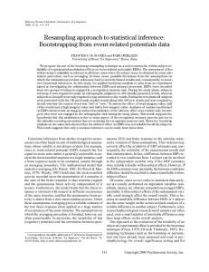
or the maximum number of iterations of 100 has been reached. The results are shown in Fig 1, were the estimated p(x|σ) for each MC simulation is shown. It is clear that the estimated Maxwellian distributions are very similar to the true density distribution. The mean value of the estimated parameter was s ^ ¼ 7:9920. The estimation from each MC simulation is shown in Fig 2. It can be clearly seen that the estimated parameter s ^ is close to the true value.

6.2 Example 2: Channel estimation in wireless communications When modelling the wireless channel, a popular technique that is commonly used corresponds to the transmission of a sine tone at a given frequency, see e.g. [68]. The received power is then modelled as a random variable. The corresponding distribution has been widely studied in the literature from measurements, and the empirical data have shown that the two most common distributions are Rayleigh an Rice [44, 45]. Hence, using similar ideas as in [50], in this example we formulate the channel distribution as a discrete sum based on a Rayleigh and a Rice component to determine the nature of the wireless channel. Table 3. Proposed algorithm for Maxwellian distribution estimation in Example 1. Step 1: i = 0. Step 2: Obtain an initial guess σ^ ðiÞ . Step 3: Compute the integral given by (66). Step 4: Compute s^ ðiþ1Þ (65) Step 5: i = i + 1 and back to Step 3 until convergence. https://doi.org/10.1371/journal.pone.0208499.t003


16 / 24


Fig 1. Estimated distribution for the stellar rotational velocity. https://doi.org/10.1371/journal.pone.0208499.g001

Fig 2. Convergence of the proposed approach to the global optimum. https://doi.org/10.1371/journal.pone.0208499.g002


17 / 24


First, the discrete mixture that we want to adjust from data is given by pðxjθÞ ¼ l1 pRayleigh ðxjs21 Þ þ l2 pRice ðxjv; s22 Þ;

ð67Þ

where pRayleigh ðxjs21 Þ

pRice ðxjv; s22 Þ

¼

¼

x e s2

x2 2s2 1

x e s21 ðx2 þv2 Þ 2s2 2

ð68Þ

;

� � xv ; s22

I0

ð69Þ

θ ¼ ½s21 ; l1 ; v; s22 ; l2 �;

ð70Þ

and I0(�) is the modified Bessel function of zeroth order. In addition, we must also include the constraint λ1+ λ2 = 1 so p(x) is a pdf. Thus, we can directly apply our proposed approach by assuming that each measurement point can be associated with a hidden variable that describes if such data point comes from the Rayleigh component or the Rice component, as it is traditionally formulated when dealing with discrete mixtures [46]. Hence, the auxiliary function Qðθ; θ^ ðiÞ Þ is given by Qðθ; θ^ ðiÞ Þ ¼

2 X 2 X

zðiÞ tj log lj þ

t¼1 j¼1

N X 2 X

zðiÞ tj log fj ðxt ; θj Þ;

ð71Þ

t¼1 j¼1

where θ^ ðiÞ is the current estimate, z is the unobserved (hidden) data and ztj is an indicator parameter such that ztj = 1 if the t-th observation comes from component j and is zero otherwise. It is given by: ðiÞ lðiÞ j fj ðxt ; yj Þ : zðiÞ ¼ P tj 2 ðiÞ ðiÞ l¼1 ll fl ðxt ; θl Þ

ð72Þ

The estimate θ^ ðiþ1Þ at the next iteration is then given by: θ^ ðiþ1Þ ¼ arg max Qðθ; θ^ ðiÞ Þ;

ð73Þ

θ

from which we obtain the following expressions: PN ^v ðiþ1Þ ¼ j

PN t¼1

½^ s 2j �ðiþ1Þ ¼

� z

ðiÞ tj

ðiÞ

t¼1

zðiÞ tj xt

I1 ðrtj Þ ðiÞ

I0 ðrtj Þ

h i x þ ^v 2j ðiÞ 2 t

^ ðiÞ 2P j ðb j Þ ^ ðiÞ P j ðb j Þ ^ ðiþ1Þ l ¼ P2 j ^ ðiÞ l¼1 P l ðb l Þ


ð74Þ

^ ðiÞ P j ðb j Þ ðiÞ

ðiÞ I1 ðrtj Þ t j I ðrðiÞ Þ 0 tj

�

2x ^v

ð75Þ

ð76Þ

18 / 24


Fig 3. Rayleigh distribution estimation using a Rayleigh-Rice mixture. https://doi.org/10.1371/journal.pone.0208499.g003

with xt ^v ðiÞ j r ¼ 2 ðiÞ ½^ sj � ðiÞ tj

^ ðiÞ P j ðb j Þ ¼

N X

ð77Þ

zðiÞ tj

ð78Þ

t¼1

We also consider the utilization of Akaike’s Information Criterion (AIC) in order to obtain an accurate yet simple model and, thus, discriminating from a Rayleigh channel, a Rice channel, and a mixture of both. With the above formulation, we consider two cases: a Rayleigh distributed channel and a Rice distributed channel. 6.2.1 Rayleigh distributed channel. In this example, the random variable x is drawn from the Rayleigh distribution � � x x2 ðTrueÞ ð79Þ pðxÞ ¼ 2 exp s 2s2 with σ2 = 1, using the Slice Sampler [69]. The best estimated model corresponds to the single Rayleigh component in the mixture. The corresponding estimation of σ2 yields s ^ 21 ¼ 1:0007 � 9:003 � 10 4 . Fig 3 shows the true Rayleigh distribution and the mean estimated pdf from the 50 MC simulations. We observe an important agreement between the true pdf and the estimated model.


19 / 24


Fig 4. Rice distribution estimation using a Rayleigh-Rice mixture. https://doi.org/10.1371/journal.pone.0208499.g004

6.2.2 Rice distributed channel. In this case, the data is drawn from the Rice distribution � 2 � x x þ v2 �xv� ðTrueÞ pðxÞ ð80Þ I0 2 ¼ 2 exp s s 2s2 with v = 4 and σ2 = 1, using the Slice Sampler. The best model is selected as a single Rician component. The corresponding estimated parameters are ^v 2 ¼ 4:003 � 1:3 � 10 3 and s ^ 22 ¼ 0:9858 � 2:2 � 10 3 . In Fig 4 we show the true Rice distribution and the mean estimated pdf from 50 MC simulations. We can observe that the estimator exhibits a good performance for the estimation of a Rice distribution.

Conclusions and future work In this paper we have presented a systematic approach for constructing surrogate functions in a wide range of inference problems. Our approach can be utilized for constructing surrogate functions for both the cost function and the constraints, generalizing the popular EM and MM algorithms. Our approach is based on the utilization of data augmentation and kernel functions, yielding simple optimization algorithms when the kernel can be expressed as VMGM. We have shown how our proposal can be utilized to solve inverse problems that are expressed as integral equations and mixture distributions. In addition, we have shown that our approach can be utilised for constrained/penalized ML and MAP estimations problems. In particular, common problems in statistical inference can directly be solved using our proposal since they can be posed as Variance Mean Gaussian Mixtures (VMGM), yielding quadratic surrogate functions.


20 / 24


In the last two decades the problem of sparse estimation has attracted a lot of attention. Since our approach can be utilized in those problems, and since it is based on the principles of the MM algorithm, a detailed analysis can be done in terms of accuracy and convergence of our technique, and compared against other techniques, such as the ones in [28, 30], and [29], where different Lasso-type problems are compared, the MM algorithm is utilized in constrained problems for ML estimation in generalized linear model regression, and the MM algorithm is used for (unconstrained) sparse estimation under non-convex penalties, respectively.

Supporting information S1 Data Set. Monte Carlo simulations for Examples 1 and 2. (ZIP)

Acknowledgments This work was partially supported by the Fondo Nacional de Desarrollo Cientı´fico y Tecnolo´gico-Chile through grants No. 3140054 and 1181158. This work was also partially supported by the Comisioń Nacional de Investigacioń Cientı´fica y Tecnolo´gica, Advanced Center for Electrical and Electronic Engineering (AC3E, Proyecto Basal FB0008), Chile. The work of R. Orellana was partially supported by the PIIC program of the Universidad Tećnica Federico Santa Marıá, scholarship 015/2018. The funders had no role in study design, data collection and analysis, decision to publish, or preparation of the manuscript.

Author Contributions Conceptualization: Rodrigo Carvajal, Juan Carlos Aguëro. Formal analysis: Rodrigo Carvajal, Juan Carlos Aguëro. Funding acquisition: Rodrigo Carvajal, Rafael Orellana, Juan Carlos Aguëro. Investigation: Rodrigo Carvajal, Dimitrios Katselis, Juan Carlos Aguëro. Methodology: Rodrigo Carvajal, Juan Carlos Aguëro. Resources: Juan Carlos Aguëro. Validation: Pedro Esca´rate. Visualization: Pedro Esca´rate. Writing – original draft: Rodrigo Carvajal, Rafael Orellana, Dimitrios Katselis, Pedro Esca´rate, Juan Carlos Aguëro. Writing – review & editing: Rodrigo Carvajal, Rafael Orellana, Dimitrios Katselis, Pedro Esca´rate, Juan Carlos Aguëro.

References 1.

Carvajal R, Aguëro JC, Godoy BI, Goodwin GC. EM-Based Maximum-Likelihood Channel Estimation in Multicarrier Systems With Phase Distortion. IEEE Trans Vehicular Technol. 2013; 62(1):152–160. https://doi.org/10.1109/TVT.2012.2217361

2.

Goldsmith A. Wireless Communications. New York, NY, USA: Cambridge University Press; 2005.

3.

Godoy BI, Goodwin GC, Aguëro JC, Marelli D, Wigren T. On identification of FIR systems having quantized output data. Automatica. 2011; 47(9):1905–1915. https://doi.org/10.1016/j.automatica.2011.06. 008


21 / 24


4.

Wang L, Zhang J, Yin GG. System identification using binary sensors. IEEE Trans Autom Control. 2003; 48(11):1892–1907. https://doi.org/10.1109/TAC.2003.819073

5.

Dempster AP, Laird NM, Rubin DB. Maximum likelihood from imcomplete data via the EM algorithm. Journal of the Royal Statistical Society, Series B. 1977; 39(1):1–38.

6.

Van Dyk DA, Meng XL. The Art of Data Augmentation. Journal of Computational and Graphical Statistics. 2001; 10(1):1–50. https://doi.org/10.1198/10618600152418584

7.

Hunter DR, Lange K. A tutorial on MM algorithms. The American Statistician. 2004; 58(1):30–37. https://doi.org/10.1198/0003130042836

8.

Pollakis E, Cavalcante RLG, Stańczak S. Base Station Selection for Energy Efficient Network Operation with the Majorization- Minimization Algorithm. In: Proc. 13th IEEE Int. Workshop on Signal Process. Adv. Wireless Commun. (SPAWC 2012). C ¸ eşme, Turkey; 2012.

9.

Figueiredo MAT, Bioucas-Dias JM, Nowak RD. Majorization–Minimization Algorithms for WaveletBased Image Restoration. IEEE Trans Image Process. 2007; 16(12):2980–2991. https://doi.org/10. 1109/TIP.2007.909318 PMID: 18092597

10.

Marks BR, Wright GP. A General Inner Approximation Algorithm for Nonconvex Mathematical Programs. Operations Research. 1978; 26(4):681–683. https://doi.org/10.1287/opre.26.4.681

11.

Aguëro JC, Tang W, Yuz JI, Delgado R, Goodwin GC. Dual time-frequency domain system identification. Automatica. 2012; 48(12):3031–3041. https://doi.org/10.1016/j.automatica.2012.08.033

12.

Beal MJ, Ghahramani Z. The Variational Bayesian EM Algorithm for Incomplete Data: with Application to Scoring Graphical Model Structures. In: Proc. of the 7th Valencia International Meeting. Valencia, Spain; 2003.

13.

Gopaluni RB. A particle filter approach to identification of nonlinear processes under missing observations. Can J Chem Eng. 2008; 86(6):1081–1092. https://doi.org/10.1002/cjce.20113

14.

Hobolth A, Jensen JL. Statistical Inference in Evolutionary Models of DNA Sequences via the EM Algorithm. Statistical Applications in Genetics and Molecular Biology. 2005; 4(1). https://doi.org/10.2202/ 1544-6115.1127 PMID: 16646835

15.

Scho¨n TB, Wills A, Ninness B. System identification of nonlinear state-space models. Automatica. 2011; 47(1):39–49. https://doi.org/10.1016/j.automatica.2010.10.013

16.

Yang S, Kim JK, Zhu Z. Parametric fractional imputation for mixed models with nonignorable missing data. Statistics and Its Interface. 2013; 6(3):339–347. https://doi.org/10.4310/SII.2013.v6.n3.a4

17.

Meng XL. Thirty Years of EM and Much More. Statistica Sinica. 2007; 17(3):839–840.

18.

Suzuki H. A Statistical Model for Urban Radio Propogation. IEEE Transactions on Communications. 1977; 25(7):673–680. https://doi.org/10.1109/TCOM.1977.1093888

19.

Cure´ M, Rial DF, Christen A, Cassetti J. A method to deconvolve stellar rotational velocities. Astronomy & Astrophysics. 2014; 565.

20.

Kraus C, Bornschein B, Bornschein L, Bonn J, Flatt B, Kovalik A, et al. Final results from phase II of the Mainz neutrino mass searchin tritium β decay. The European Physical Journal C—Particles and Fields. 2005; 40(4):447–468.

21.

Semkow TM, Li X. Application of integral equations to neutrino mass searches in beta decay; 2018. ArXiv e-prints. Available from: http://adsabs.harvard.edu/abs/2018arXiv180105009S.

22.

Polson NG, Scott JG. Data augmentation for non-Gaussian regression models using variance-mean mixtures. Biometrika. 2013; 100:459–471. https://doi.org/10.1093/biomet/ass081

23.

Barndorff-Nielsen O, Kent J, Sorensen M. Normal variance-mean mixtures and z distributions. Int Stat Review. 1982; 50(2):145–159. https://doi.org/10.2307/1402598

24.

West M. On scale mixtures of normal distributions. Biometrika. 1987; 74(3):646–648. https://doi.org/10. 1093/biomet/74.3.646

25.

Balakrishnam N, Leiva V, Sanhueza A, Vilca F. Estimation in the Birnbaum-Saunders distribution based on scale-mixture of normals and the EM algorithm. SORT. 2009; 33(2):171–192.

26.

Carvajal R, Aguëro JC, Godoy BI, Katselis D. A MAP approach for ℓq-norm regularized sparse parameter estimation using the EM algorithm. In: Proc. of the 25th IEEE Int. Workshop on Mach. Learning for Signal Process (MLSP 2015). Boston, USA; 2015.

27.

Godoy BI, Aguëro JC, Carvajal R, Goodwin GC, Yuz JI. Identification of sparse FIR systems using a general quantisation scheme. Int J Control. 2014; 87(4):874–886. https://doi.org/10.1080/00207179. 2013.861611

28.

Yuan M, Lin Y. Model selection and estimation in regression with grouped variables. Journal of the Royal Statistical Society, Series B. 2006; 68(1):49–67. https://doi.org/10.1111/j.1467-9868.2005. 00532.x


22 / 24


29.

Fan J, Liu H, Sun Q, Zhang T. I-LAMM for sparse learning: Simultaneous control of algorithmic complexity and statistical error. Ann Statist. 2018; 46(2):814–841. https://doi.org/10.1214/17-AOS1568

30.

Xu J, Chi E, Lange K. Generalized Linear Model Regression under Distance-to-set Penalties. In: Proc. of 30th Neural Information Processing Systems Conference. Barcelons, Spain; 2016. p. 1385–1395.

31.

Durret R. Probability: Theory and examples. 4th ed. Cambridge University Press; 2010.

32.

Akaike H. A new look at the statistical model identification. IEEE Trans Aut Control. 1974; 19(10):716– 723. https://doi.org/10.1109/TAC.1974.1100705

33.

McLachlan GJ, Krishnan T. The EM Algorithm and Extensions. Wiley; 1997.

34.

Vaida F. Parameter convergence for EM and MM algorithms. Statistica Sinica. 2005; 15(3):831–840.

35.

Sriperumbudur BK, Torres DA, Lanckriet GRG. A majorization-minimization approach to the sparse generalized eigenvalue problem. Machine Learning. 2011; 85(1–2):3–39. https://doi.org/10.1007/ s10994-010-5226-3

36.

Tanner MA. Tools for Statistical Inference: Observed Data and Data Augmentation Methods. Springer; 1991. https://doi.org/10.1007/978-1-4684-0510-1

37.

Figueiredo MAT. Adaptive sparseness for supervised learning. IEEE Trans Pattern Anal Mach Intell. 2003; 25(9):1150–1159. https://doi.org/10.1109/TPAMI.2003.1227989

38.

Park T, Casella G. The Bayesian Lasso. Journal of the American Statistical Association. 2008; 103 (482):681–686. https://doi.org/10.1198/016214508000000337

39.

Garrigues P, Olshausen B. Group sparse coding with a laplacian scale mixture prior. Advances in Neural Information Processing Systems. 2010; 23:676–684.

40.

Wazwaz AM. Linear and Nonlinear Integral Equations: Methods and Applications. Springer; 2011.

41.

Christen A, Escarate P, Cure´ M, Rial DF, Cassetti J. A method to deconvolve stellar rotational velocities II. Astronomy & Astrophysics. 2016; 595(A50):1–8.

42.

Chandrasekhar S, Mu¨nch G. On the Integral Equation Governing the Distribution of the True and the Apparent Rotational Velocities of Stars. Astrophysical Journal. 1950; 111:142–156. https://doi.org/10. 1086/145245

43.

Molisch A. Wireless Communications. Wiley-IEEE Press; 2005.

44.

Salous S. Radio Propagation Measurement and Channel Modelling. Wiley; 2013.

45.

Pa¨tzold M. Mobile Radio Channels. Wiley; 2011.

46.

Mengersen KL, Robert C, Titterington M. Mixtures: Estimation and Applications. Wiley; 2011.

47.

McLachlan G, Peel D. Finite Mixture Models. Wiley; 2004.

48.

DeGroot M. Optimal statistical decisions. New York, NY, USA: McGraw-Hill; 1970.

49.

Redner RA, Walker HF. Mixture Densities, Maximum Likelihood and the EM Algorithm. SIAM Review. 1984; 26(2):195–239. https://doi.org/10.1137/1026034

50.

Orellana R, Carvajal R, Aguëro JC. Maximum Likelihood Infinite Mixture Distribution Estimation Utilizing Finite Gaussian Mixtures. In: 18th IFAC Symposium on System Identification (SYSID). Stockholm, Sweden; 2018.

51.

Goodwin GC, Payne RL. Dynamic system identification: experiment design and data analysis. Academic Press New York; 1977.

52.

So¨derstro¨m T, Stoica P, editors. System Identification. Upper Saddle River, NJ, USA: Prentice-Hall, Inc.; 1988.

53.

Ljung L, Goodwin GC, Aguëro JC. Stochastic Embedding revisited: A modern interpretation. In: Proc. of the 53rd IEEE Conf. Decision and Control). Los Angeles, CA, USA; 2014.

54.

Mahata K, So¨derstro¨m T. Improved estimation performance using known linear constraints. Automatica. 2004; 40(8):1307–1318. https://doi.org/10.1016/j.automatica.2004.03.001

55.

Lange K. Optimization. 2nd ed. New York, USA: Springer; 2013.

56.

Hanson MA. Inequality constrained maximum likelihood estimation. Ann Inst Stat Math. 1965; 17 (1):311–321. https://doi.org/10.1007/BF02868175

57.

Hyder MM, Mahata K. A Robust Algorithm for Joint-Sparse Recovery. Signal Process Letters, IEEE. 2009; 16(12):1091–1094. https://doi.org/10.1109/LSP.2009.2028107

58.

Grant MC, Boyd SP. Graph Implementations for Nonsmooth Convex Programs. In: Blondel VD, Boyd SP, Kimura H, editors. Recent Advances in Learning and Control. London: Springer; 2008. p. 95–110.

59.

Lemieux C. Monte Carlo and Quasi-Monte Carlo Sampling. New York, NY, USA: Springer; 2009.

60.

Press WH, Teukolsky SA, Vetterling WT, Flannery BP. Numerical Recipes: The Art of Scientific Computing. 3rd ed. Cambridge University Press; 2007.


23 / 24


61.

Tibshirani R. Regression shrinkage and selection via the lasso. J Royal Statist Soc B. 1996; 58(1):267– 288.

62.

Zou H, Hastie T. Regularization and variable selection via the elastic net. Journal of the Royal Statistical Society, Series B. 2005; 67:301–320. https://doi.org/10.1111/j.1467-9868.2005.00503.x

63.

Li Q, Lin N. The Bayesian elastic net. Bayesian Anal. 2010; 5(1):151–170. https://doi.org/10.1214/10BA506

64.

Fletcher R. Practical methods of optimization. 2nd ed. Chichester, GB: John Wiley & Sons; 1987.

65.

Izmailov AF, Solodov MV. Newton-type methods for optimization and variational problems. Cham, Switzerland: Springer; 2014.

66.

Deutsch AJ. Maxwellian distributions for stellar rotation. In: Proc. of the IAU Colloquium on Stellar Rotation. Ohio, USA; 1969. p. 207–218.

67.

Robert CP, Casella G. Monte Carlo statistical methods. Springer, New York; 1999.

68.

Rodrı´guez M, Feick R, Carrasco H, Valenzuela R, Derpich M, Ahumada L. Wireless Access Channels with Near-Ground Level Antennas. IEEE Transactions on Wireless Communications. 2012; 11 (6):2204–2211. https://doi.org/10.1109/TWC.2012.041612.110735

69.

Neal RM. Slice sampling. Ann Statist. 2003; 31(3):705–767. https://doi.org/10.1214/aos/1056562461


24 / 24