data producers. These new approaches allow students to maintain better focus on the big ideas of statistics. These new approaches are a great step forward for ...
JSM2015 - Section on Statistical Education
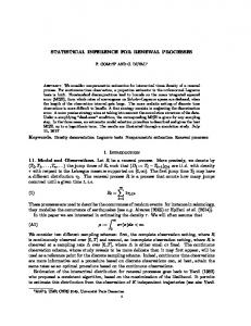
STATISTICAL INFERENCE FOR MANAGERS Milo Schield, W. M. Keck Statistical Literacy Project. Minneapolis, MN. Abstract: Managers are defined as those in management, marketing, international business and management information systems. Managers are estimated to be at least 20% of the undergraduates taking introductory statistics at four-year colleges. This paper claims that the statistical-inference needs of managers are quite different from the needs of the others taking introductory statistics. Most other students taking introductory statistics are expected to read journal articles involving statistical studies and statistical inference. They may even be expected to conduct a statistical study. Managers seldom – if ever -- read research articles involving statistical studies. They are not expected to conduct a statistical study. Their job is to use statistics to make better decisions. They do need to recognize the influence that chance can have on their data. They do need to realize that statistics and statistical associations can be influenced by confounders and by how statistics are defined, counted and measured. They do need separate skill from luck, to separate what is most likely from what is quite probable. By studying statistical inference (confidence intervals and statistical significance) they are being sensitized to the role of chance in their field and to the fact that statistics exist in a context where the context matters. Managers do not need to understand the logic or derivation of the sampling distribution, the central limit theorem, the details of hypothesis testing or the calculation or meaning of p-values. Statistical inference for managers will involve a small deviation from a few of the GAISE supplementary goals. Making these changes may increase their understanding of statistical significance. Making these changes will allow room for other important topics such as multivariate data, confounding and coincidence. Keywords: Statistical literacy, statistical significance, statistical education, effect sizes 1. Students Taking Introductory Statistics by Major The statistical inference needs for students taking statistics vary by major. Appendix A examines the distribution by major. Business-Economics majors are estimated to be 40% of undergraduates taking introductory statistics at US four-year colleges. Since Business-Economics is the largest category, it is helpful to divide businesseconomics majors into two groups: quantitative (Economics, Finance and Accounting) and qualitative (Management, Marketing, International and MIS). This is fairly crude since some Marketing and MIS majors focus on surveys and analytics. We are unaware of any statistics on the percentage of Business-Economics majors that are in each group. For simplicity, 50-50 was used. At Augsburg the percentage of Business-Economics graduates who are in qualitative majors has been between 60% and 70% since 2003. Figure 1: Estimated Distribution of US College Students Taking Statistics by Major
Henceforth those business students in qualitative majors will be referred to as managers. On that basis, managers are 20% of those taking introductory statistics. This paper
3032
JSM2015 - Section on Statistical Education
argues that the statistical inference needs of managers are quite different from the statistical inference needs of all the other groups required to take statistics. One way to quickly see the difference is to survey majors on their choice of statistical software. Managers typically use Excel. All other groups use statistical software or Excel with add-ins: SPSS for those in Sociology and Psychology, R for those in Mathematics, and Minitab or Excel with add-ins for those in Economics and Finance. JMP and SAS are used throughout the social sciences and professions. (Phelps and Szabat, 2015) Appendix B reviews recent pedagogical advances in teaching introductory statistics to data producers. These new approaches allow students to maintain better focus on the big ideas of statistics. These new approaches are a great step forward for statistical education. But they are not enough for Managers. 2. Statistical Inference Needs of Business Managers Business managers have some of the same needs for statistical inference as does everyone else taking an introductory statistics course: they should be exposed to the major contributions of statistics to human knowledge. Figure 2 shows the Schield (2015) choices: the big ideas that all students taking statistics should know. The goal is to teach these big ideas with as little overhead – as little baggage – as possible. Figure 2: Major Contributions of Statistics to Human Knowledge.
Managers have very different needs from the statistical producers. Managers seldom encounter statistical studies in journals. Consumers and employees are not readily assigned to be subjects in experiments. Managers are much more likely to read case studies such as those in the Harvard Business Review. Almost all these cases are observational studies. Industry and social statistics are common so the data is typically multivariate. References to statistical inference are rare except in surveys. Yet statistics and statistical comparisons are common. Managers must evaluate the meaning and reliability of these statistics; they must evaluate the strength of evidence provided by these statistics to make good business decisions.
3033
JSM2015 - Section on Statistical Education
Before pressing on with the observation that managers seldom read statistical studies in journals, it is important to give reason why this practice is appropriate. Managers are not looking to find "truths" about people. They are pragmatic. People have different skills, attitudes, needs and wants. And these change. Managers want to know what techniques will make a big difference. "Does it work?" is an ongoing question. Managers deal with quasi-experiments when they change prices, discounts, commissions, wages, advertising, etc. Managers are constantly trying to untangle the overlap between luck and skill (Mauboussin, 2012). Some association may be true, but if their effect sizes are too small, the connections may not be worth implementing. This managerial focus on practicality and large effect sizes means that with even small sample sizes the large effects will generally be statistically-significant – and be resilient to the influence of potential confounders. They also must deal with coincidence. Chance has many forms and yet is often ignored as a source of influence on statistics. This paper makes five claims: (1) Managers need basic statistical literacy: sampling error, margin of error, confidence intervals, the idea of statistical significance, the understanding that the non-overlap between paired 95% confidence intervals is sufficient for statistical significance. (2) Managers need to be exposed to the formulas for the 95% margin of error so they see how it relates to sample size. They need this to understand the survey margin of error commonly provided for most surveys so they can adjust it for survey subgroups and for small probabilities. (3) Managers need to understand that confounding in observational studies can influence the size of the statistics and the statistical significance of an association. They need to understand that random assignment statistically controls for all pre-existing confounders and gives strong support for causation. (4) Managers need to understand the idea of hypothesis testing, the privileged status of the null hypothesis, and the difference between Type1 and Type 2 error. These ideas are applicable in everyday life and in business. When confidence intervals are not available, they need simple sufficient shortcuts for what size associations are sufficient for statistical significance. These associations should go beyond simple differences to include correlations, chi-square and the t-statistic. (5) Managers do not need to understand – or even see – the logical chain by which the central limit theorem is justified, the details of a sampling distribution, the details of hypothesis testing or p-values – contrary to the GAISE supplementary goals. They do not need to deal with one-tail versus two tail tests or with one-sample tests. This eliminates a fair amount of the material in most introductory textbooks. This gives room to add many non-inference topics involving big data that are of increasing importance to managers such as confounding and coincidence. (Schield 2014). Schield (2004) reported evidence that those in business seldom encounter hypothesis tests. Fidler (2006) argues for replacing p-values with confidence intervals. Schield (2013) argued that managers need a different statistics course that focuses on "statistical thinking, hypothetical thinking, evaluative thinking and judgmental thinking." "Of all the courses in the business core, introductory statistics is most in need of reinvention. Requiring business students in non-quantitative majors to spend an entire course
3034
JSM2015 - Section on Statistical Education
studying the statistics of random samples is unnecessary and unproductive." "Those teaching business have an obligation to prepare their students for practice. The faculty teaching business statistics have the same obligation. If sample-based statistical inference is almost as distant as cost accounting from the needs of most business students in non-quantitative majors, then those teaching business statistics must find new options." Appendix C present ways of teaching statistical inference using just margin of error and confidence intervals. Topics include the complexity beneath the typical survey margin of error (C1), teaching statistical significance using non-overlapping confidence intervals. (C2), teaching the relationship between statistical significance, confounding, random assignment and causation (C3), teaching statistical significance in place of p-values (C4), and the other benefits of teaching introductory statistics using confidence intervals (C5). If using the absence of overlap in 95% confidence intervals is not adequate or appropriate, appendix D presents some shortcuts in determining statistical significance (van Belle, 2008). Appendix D includes these statistically-significant shortcuts: Z-statistic for proportions (D1), independent correlations (D2), Chi-squared (D3), and the t-statistic (D4). D5 discusses obtaining a statistically-significant shortcut for serial correlation. 3. Challenges in Offering Statistics for Managers Any curricular change has benefits and costs. Before making the changes suggested above, it is important to note some of the challenges. Students may not have chosen their major within business – or they may change their major from manager (qualitative) to quantitative. Students within management-marketing may have strong quantitative skills, aptitude and interest. Finally, teacher training for a substantially different course may be problematic. Some statistical educators may be unwilling. At Augsburg, students majoring in Management, Marketing, International Business or MIS can choose between the traditional introductory statistics course and the Statistics for Managers course. Students in Economics, Finance and Accounting are required to take the traditional introductory statistics course. Augsburg students taking Statistics for Managers are generally pleased with the greater emphasis on reading, interpreting and communicating statistics – and the focus on Excel. They generally see value in what they are studying. 4. Conclusion Teachers, textbook authors and publishers need to recognize that managers have very different statistical needs from others taking statistics. Managers have needs that are broader: multivariate data, confounding, coincidence, etc. With the advent of big data, these other needs are even more demanding. Managers don't need the precision taught to others taking statistics. Providing mathematical exactness may inadvertently make perfection (deductive certainty) the enemy of the good. Although de-emphasizing the sampling distribution, p–values and one-population hypothesis tests may undercut some of the GAISE supplementary goals, doing so might actually improve students understanding of statistical significance. A secondary justification is that it would provide room for other important statistical topics such as confounding and coincidence. Achieving both of these goals could make a big improvement in the education of business managers.
3035
JSM2015 - Section on Statistical Education
REFERENCES Cumming, Geoff (2012). Understanding the New Statistics: Effects Sizes, Confidence intervals, and Meta-Analysis. Routledge Digest of Education Statistics (2013). nces.ed.gov/programs/digest/2013menu_tables.asp Fidler, F. (2006). Should Psychology abandon p values and teach CIs instead? ICOTS 7. See https://www.stat.auckland.ac.nz/~iase/publications/17/5E4_FIDL.pdf Giere, R., J. Bickle, R. Mauldin (2005). Understanding Scientific Reasoning. Wadsworth. Hoekstra, R. (2014). The interpretation of effect size. ICOTS 9. http://icots.info/9/proceedings/pdfs/ICOTS9_6B3_HOEKSTRA.pdf
Copy at
Mauboussin, M. (2012). The Success Equation: Untangling Skill and Luck in Business, Sports, and Investing. Harvard Business Review Press Moore, D. (1997). Statistical Literacy and Statistical Competence in the 21st Century [slides]. www.statlit.org/pdf/1997MooreASAslides.pdf Phelps, Amy and Kathryn Szabat (2015). Current Landscape of Business Analytics and Data Science at Higher Education Institutions: Who is Teaching What? Copy at www.statlit.org/pdf/2015-Phelps-Szabat-ASA-Slides.pdf Ramsey, F. and D. Schaffer (2002). The Statistical Sleuth. 2nd ed. Duxbury. Raymond, R. and M. Schield (2008). Numbers in the News: A Survey. 2008 Proceedings of the Section on Statistical Education. P 14-18. Copy at www.statlit.org/pdf/2008RaymondSchieldASA.pdf Rossman, A. (2007). Seven Challenges for the Undergraduate Statistics Curriculum in 2007. USCOTS Plenary. See www.statlit.org/pdf/2007RossmanUSCOTS6up.pdf Schield, Milo (2004). Statistical Literacy Curriculum Design. IASE Curricular Development in Statistics. Statistics Education Roundtable, Sweden. Copy at www.statlit.org/pdf/2004SchieldIASE.pdf Schield, M. (2006). Presenting Confounding and Standardization Graphically. STATS, ASA. Fall 2006. pp. 14-18. Copy at www.StatLit.org/pdf/2006SchieldSTATS.pdf Schield, M. and C. Schield (2007). Numbers in the News: A Survey. ASA Proceedings of the Section on Statistical Education. See www.statlit.org/pdf/2007SchieldASA.pdf Schield, M. (2010). Assessing Statistical Literacy: TAKE CARE in Assessment Methods in Statistical Education: An International Perspective. Hunt and Joliffe, Eds. Excerpts: www.statlit.org/pdf/2010SchieldExcerptsAssessingStatisticalLiteracy.pdf Schield, M. (2013). Reinventing Business Statistics: Statistical Literacy for Managers. MBAA Chicago. Copy at www.statlit.org/pdf/2013-Schield-MBAA.pdf Schield, M. (2014). Two Big Ideas for Teaching Big Data. Electronic Conference on Teaching Statistics (E-COTS). www.statlit.org/pdf/2014-Schield-ECOTS.pdf Schield, M. (2015). What is Wrong with the Introductory Course. US Conference on Teaching Statistics (USCOTS). See www.statlit.org/pdf/2015-Schield-USCOTS.pdf Sharpe, N., R. DeVeaux and P. Velleman (2011) Business Statistics: A First Course. Utts, J. (2014). Seeing Through Statistics. Fourth edition. Wadsworth Publishing. van Belle, G. 2008. Statistical Rules of Thumb. Wiley.
3036
JSM2015 - Section on Statistical Education
Appendix A: Students Taking Introductory Statistics by Major The statistical needs of those taking statistics is highly dependent on their major. Unfortunately, there is no data on which students are taking statistics, but this can be estimated based on graduates by major and which majors typically require their students to take statistics. This estimate assumes all those taking Business & Economics, Sociology & Social Work, Health Sciences, Psychology and Biology are required to take introductory statistics. Of the 1.79 million US BA/BS graduates from four-year colleges in 2011, an estimated 914,000 (51%) took statistics. (Digest of Education Statistics, 2013). This estimate ignores students taking statistics to satisfy a general education or quantitative reasoning requirement. It also ignores the 2% of college graduates majoring in statistics, MBA graduate students and those at two-year colleges taking statistics. If those were included, over half of those taking statistics at the college level are majoring in Business and Economics. Figure 1 estimates the distribution by major of US four-year college undergraduates taking statistics. Figure 3: Distribution of US College Students Taking Statistics by Major
Appendix B: Statistical Needs of Data Producers David Moore (1997) distinguished statistical literacy (for consumers) from statistical competence (for producers). Most students required to take statistics are data producers. Data producers are expected to read research papers and to conduct studies in which statistical inference and p-values are common. Introductory textbooks for data producers typically present the logic and derivation of the Central Limit Theorem. While this provides mathematical rigor, it may divert attention from the big ideas in statistics. In addition to presenting the derivation of the central limit theorem, most introductory textbooks present a comprehensive coverage of the various types of statistical tests. Although two-population tests are most common in the literature and in practice, onepopulation tests are typically presented as a pedagogical introduction. This extensive coverage is presumably justified for those students that will read or conduct statistical studies. This extensive coverage generally occupies a significant portion of an introductory statistics textbook – and of an introductory statistics course. Providing this comprehensive coverage of hypothesis tests has a disadvantage. As Rossman (2007) noted, "You simply can’t achieve these [GAISE statistical literacy] goals in one course if you also teach a long list of methods." He suggested that "Most students would be better served by a Stat 100 [statistical literacy] course than a Stat 101 [methods] course." Some recent introductory statistics textbooks have blazed a trail for bypassing the full derivation of the central limit theorem.
3037
JSM2015 - Section on Statistical Education
•
•
•
Sharpe, DeVeaux and Velleman (2011) omit the traditional derivation of the central limit theorem. Based on a simulation, they note that the shape of this sampling distribution is approximately Normal. They introduce a formula for the standard deviation of the sampling distribution of proportions. After testing the simulation against a Normal model, they state "So, the particular Normal model, N(p, Sqrt(p*q/n)) is a sampling distribution model for the sample proportion." They conclude by saying "this model can be justified theoretically with just a little mathematics." They do present the Central Limit theorem for proportions (page 261) and for means (page 322). Utts (2014) goes even further in bypassing the full logic behind the derivation of a sampling distribution. On page 412, the sampling distribution for proportions is introduced as the "Rule for sample proportions" saying "The following is what statisticians have determined to be approximately true …" On page 416, under "Defining the Rule for Sample Means", she states, "The Rule for Sample Means is simple: …." A further sign that the central limit theorem has been downgraded is that the phrase "central limit theorem" does not even appear in the index. Utts (2014) included p-values, but gave less attention to their derivation while giving more attention to interpreting p-values in journal articles. Appendix C: Statistical Inference Needs of Managers
C1. Understanding the survey margin of error. Next to "statistical significance", "margin of error" is the most common sign of statistical inference in the everyday media. (Schield and Schield 2007; Raymond and Schield 2008). Most high-quality surveys state the margin of error. We call this “the survey margin of error”. Data consumers need to recognize that (1) this survey margin of error is for the entire sample – not for any of the subgroups, and (2) this survey margin of error is the maximum margin of error possible in a sample the size of the survey. This survey margin of error is computed assuming the chance of success is 50%. Data consumers need to know how to adjust this survey margin of error for subgroups. Say the sample is half men, half women. The size-adjusted margin of error for either group would be the survey margin of error times the square-root of two: a larger number. Data consumers need to know how to adjust this survey margin of error when the percentages are very different from 0.50. Suppose the survey provides the percentage of respondents who have done hard drugs with an overall value of 10%. The chanceadjusted margin of error would be the survey margin of error times square-root of [(0.1*0.9) / (0.5*0.5)]: a smaller number. Data consumers need to know how to generate confidence intervals given a margin of error. Although this may seem like a trivial matter, it is essential in order to test for statistical significance using non-overlapping confidence intervals. C2. Statistical Significance using Non-Overlapping Confidence Intervals Data consumers need to know whether an association between two statistics is statistically significant. Giere et al. (2005) argue that the idea of statistical significance is most quickly and easily introduced to non-statisticians by the non-overlap of paired 95%
3038
JSM2015 - Section on Statistical Education
confidence intervals. Cumming (2012) provides a wealth of insight into the value of – and the misconceptions of – confidence intervals. Statistical educators are well-aware that statistical significance at the 0.05 level is guaranteed if two paired 95% confidence intervals do not overlap. This is an extremely simple way to introduce statistical significance. However few – if any – introductory statistics textbooks present this idea. Here are two good reasons for not using this approach: •
•
The p-value associated with two 95% confidence intervals that just touch is much less than 0.05. Thus, a non-overlap between two 95% confidence intervals is sufficient – but not necessary – for statistical significance. Two paired 95% confidence intervals may overlap and yet the difference in their sample statistics may still be statistically significant. The basic elements of hypothesis testing are hidden. There is no distinction between a one-tailed and a two-tailed test with confidence intervals. The power of a statistical test is not available when using confidence intervals. There is no way to access a p-value.
These are important reasons to avoid using non-overlapping confidence intervals as a sufficient condition for statistical significance. But for managers, the simplicity and the accessibility of confidence intervals arguably outweighs the negatives listed above. Furthermore, this confidence-interval approach provides a simple way of demonstrating that statistical significance can be influenced by confounding. C3. Statistical significance, confounding, random assignment & causation Here is another reason for using confidence intervals. Statistical significance can be influenced by confounding and assembly (how things are defined, grouped or measured). This is easily demonstrated using confidence intervals. (Schield, 2004, 2006) Figure 4: Confounder Influence on Statistical Significance: Before vs. After
As shown in the left graph, smokers are more likely to be younger moms, so younger moms are more likely to smoke. Younger moms are more likely to have low birth-weight babies. The mom's age is a relevant confounder. Controlling for the mom's age by standardizing in the right graph transforms a statistically-significant difference into one that is not statistically significant. Students taking a traditional statistics course never see that
3039
JSM2015 - Section on Statistical Education
statistical significance can be influenced by confounding. Managers need to see this in order to make good decisions. (Schield, 2010). When subjects are randomly assigned to treatment and control groups, this statisticallycontrols for pre-existing confounders. If the resulting association is statistically significant, this supports the claim that the treatment caused the result. C4. Teaching Statistical Significance in place of P-values Excluding p-values is a big change. Most – if not all – introductory statistics textbooks feature p-values. Statistical significance may be mentioned, but often the mention is dismissive. Selecting a single cutoff (5%) is arbitrary. A single-cutoff does not distinguish barely significant (0.05) from highly significant (0.005); it unfairly distinguishes between barely insignificant (0.051) from barely significant (0.05). But there are two ways in which something can be arbitrary. One way is that something can be anything. A second way is that something can be anything but within a very narrow range. This argument over the arbitrary tends to mask a big idea: the difference between statistically significant (very small p-value) and statistically insignificant (a large p-value). Once again the ideal – the exact – may become the enemy of the good – the understanding of an important difference. P-values are seldom – if ever – found in business case studies or encountered by business managers. Furthermore introducing p-values may have collateral damage. Students may leap to the unwarranted conclusion that the p-value is the chance the null is true. Students get confused by the idea that "smaller is bigger": the smaller the p-value, the more statistically significant is the relationship. Since managers seldom read statistical studies, they do not need to understand the full logic behind the derivation of the central limit theorem, the relation between the t-statistic and degrees of freedom, the detailed setup of hypothesis testing, the calculation and interpretation of p-values, one-sided versus two-sided tests or the power of a test. Managers need to have a clear understanding of statistical significance and its relationship to sample size. They need to have a clear understanding of what is means for a statistic or a statistical association to lack statistical significance: to be statistically insignificant. They need to understand the difference between a significant difference, an important difference and an undetected difference: the difference between no relationship and no statistically-significant relationship. They need to think clearly about whether and when being statistically significant is strong evidence in favor of a difference. They need to understand the epidemiological justification for causation in observational studies. They need to think clearly about whether and when being statistically significant is strong evidence in favor of causation. If the goal is to help managers understand important ideas – such as statistical significance – it may be appropriate to forego any reference to p-values. Statistical significance should be introduced as being statistically unlikely. Here are some ways that statistical significance can introduced at the start of an introductory statistics course: 1. What is the chance of a run of heads? At what length run does the event become statistically-significant? Too, three, four, five or six heads? By setting statistical
3040
JSM2015 - Section on Statistical Education
significance as less than a 5% probability, we can see that getting heads on each of the next five randomly flipped coins would be statistically significant. 2. For a six-sided die, the chance of getting a pre-specified side on the next roll is one chance in six. Getting two such events on the next two fair rolls would be statistically significant. C5. Other Benefits of teaching statistical inference using confidence intervals Aside from being intuitive and accessible, there are two other reasons for using nonoverlapping confidence intervals as a sufficient condition for statistical significance. 1. Confidence intervals are related to effect size. Effect size is a most important idea. (Hoekstra, 2014) Larger effect sizes are more likely to resist the influence of confounders. A p-value does not provide any indication of effect size. . 2. Using confidence intervals as a test for statistical significance allows students to work problems involving a binary confounder. Students can see how controlling for a confounder can transform a statistically-significant association into one that is statistically-insignificant – and vice versa. See Schield (2004, 2006, 2010). Appendix D: Statistical Significance Shortcuts D1. Statistical Significance Shortcuts for a Test of Proportions A conservative shortcut for statistical significance is given by 1/Sqrt(n). The complete form for a 95% margin of error is 1.96 Sqrt[p*(1-p)/n] where p(1-p) is a maximum at p = 0.5, so the shortcut conservative form becomes 1/Sqrt(n). D2. Statistical-Significance Shortcut for Independent Correlations SUMMARY: Testing a correlation for statistical significance is not easy. The detail below notes three ways of obtaining the sampling distribution from a bivariate normal. None of these are easy or memorable without statistical software. A simple short-cut sufficient condition for statistical significance is given by r > 2/sqrt(n). As shown in Figure 4, this shortcut is always greater than the exact value but is within 5% of the exact value for n between four and 1,600. Figure 5: Statistically-Significant Correlation Coefficients versus Sample Size
3041
JSM2015 - Section on Statistical Education
DETAIL: The distribution of correlations for random selections from an uncorrelated bivariate Normal is not easily obtained or described without statistical software. Here are three analytic approaches: 1. Fisher transformation using Ln() and Arctanh(), 2. an exact solution using a Gamma function, or 3. Student-t distribution: t = r*Sqrt[(n-2)/(1-r^2)]; df = n-2 None of these are simple or memorable. Instead of requiring an exact solution for the sampling distribution, look for a sufficient condition for a statistically-significant correlation that is simple and memorable. 1. For a wide range of sample sizes (n), find the smallest value of r that is statistically significant. Using the calculator at www.vassarstats.net/rho.html, find the smallest four-digit value of r where the p-value is no more than 0.05. Using the calculator at www.danielsoper.com/statcalc3/calc.aspx?id=44, find the smallest four-digit value of r where the left-end of the 95% confidence interval is at least zero. There are some very slight differences between these two calculators. For n = 5, r = 0.88, Vassar indicates statistical significance (p = 0.0456) while Daniels shows the opposite (lower end of 95% confidence interval is -0.01). 2. Try different models that fit these minimum statistically-significant correlations. Choose the simplest that is sufficient over a wide range. Measure the accuracy. Consider the results of this simple model: R = 2/Sqrt(n). There are two ways to assess the model: #1: Error in correlation (r) for a given sample size (n) or #2: Error in sample size (n) for a given correlation (r). The following table uses #1: it gives the percentage error in the correlation for a given sample size. Table 1. Modelling Statistical Significance for Independent Correlations N 1600 900 400 256 100 49 25 16 9 8 7 6 4
Model 2/sqrt(n) 0.0500 0.0667 0.1000 0.1250 0.2000 0.2857 0.4000 0.5000 0.6667 0.7071 0.7559 0.8165 1.0000
Min S/S Min S/S Vassar Daniels 0.0481 0.0491 0.0644 0.0654 0.0971 0.0981 0.1217 0.1227 0.1955 0.1966 0.2803 0.2816 0.3943 0.3961 0.4950 0.4974 0.6636 0.6664 0.7042 0.7068 0.7527 0.7545 0.8113 0.8115 0.9611 0.9500
% Error % Error Vassar Daniels 3.95% 1.83% 3.52% 1.94% 2.99% 1.94% 2.71% 1.87% 2.30% 1.73% 1.93% 1.46% 1.45% 0.98% 1.01% 0.52% 0.46% 0.04% 0.41% 0.04% 0.43% 0.19% 0.64% 0.62% 4.05% 5.26%
Note that all errors are positive. Correlations at least as big as the model values are guaranteed to be statistically-significant. Smaller correlations may be statisticallysignificant.
3042
JSM2015 - Section on Statistical Education
D3. Statistical Significance Shortcut for Chi-Squared SUMMARY: Testing for statistical significance in a given value of chi-squared normally requires access to a table or a function. Neither is easy or memorable. The detail below presents a shortcut criteria for statistical significance: Chi-square = 2*(DF + 1). Any value of chi-square with at least this value is guaranteed to be statisticallysignificant. This sufficient condition is very accurate for DF < 5 since error increases as DF increases. Figure 6: Statistically-Significant Chi-Square versus Degrees of Freedom
Since most tests of independence involve a 2xC table, these tables have DF = C-1. Thus, this modelled shortcut, 2*(DF+1), becomes 2*C. If a two-group chi-square is at least 2*C, then it is guaranteed to be statistically significant. This relationship is simple and memorable. DETAIL: The chi-square distribution is the sum of the squares of k independent standard normal random variables. It is not simple or memorable. This approach is to find the minimum values of chi-square that are statistically-significant for various degrees of freedom (DF) and see if those values can be modelled by something simple and memorable. Excel makes it very easy to obtain the minimum value of chi-squared that is statistically significant for a given DF using this Excel function: =CHISQ.INV.RT(0.05, DF) Although the chi-squared test is a two tailed test, chi-squared is always positive, so the pvalue is just the area in the upper-right tail. This test requires that each cell have at least a count of five. If some cells do not satisfy that requirement, then the two cells with the lowest count should be combined until this condition is satisfied. One model, 2*(DF + 1), emerged as both simple and fairly accurate for DF < 5. The following table shows the exact chi-square cutoff, the model cutoff and the error.
3043
JSM2015 - Section on Statistical Education
Table 2. Modelling Statistical Significance for Chi-Square Degrees Chi-square Chi-sq Freedom Cutoff/Min Y=2(DF+1) 1 3.84 4.00 2 5.99 6.00 3 7.81 8.00 4 9.49 10.00 5 11.07 12.00 6 12.59 14.00 7 14.07 16.00 8 15.51 18.00 9 16.92 20.00 10 18.31 22.00 11 19.68 24.00 12 21.03 26.00 13 22.36 28.00 14 23.68 30.00 15 25.00 32.00 19 30.14 40.00 30 43.77 62.00 40 55.76 82.00 45 61.66 92.00
20%
Error: Model vs. Exact
Error 4.1% 0.1% 2.4% 5.4% 8.4% 11.2% 13.7% 16.1% 18.2% 20.2% 22.0% 23.7% 25.2% 26.7% 28.0% 32.7% 41.6% 47.1% 49.2%
Statistically-Significant Chi-Square Error
15%
Model: 2(DF+1)
10% 5% 0%
1
3
5 Degrees of Freedom
7
9
For 4 < DF < 20, a more accurate but more complex model is 4 + 1.5*(DF+1). Minimum Statistically-Significant Chi-Square Error: Actual vs. Linear Model II
50%
Model II: 4 + 1.5 *DF
40% 30% 20% 10% 0%
1
3
5
7
9 11 13 Degrees of Freedom
15
17
19
In a table with R rows and C columns, degrees of freedom (DF) is given by (R-1)(C-1). For a 2x2 table, there is just one degree of freedom. For a two by R table, there are R-1 degrees of freedom. Many – if not most – student exercises involve DF < 5. D4. Statistical Significance Shortcut for a T-Statistic SUMMARY: The t-statistic is highly dependent on the sample size. The t-statistic approaches Z as the sample size increases. The following investigates two different models for a statisticallysignificant t-statistic: a difference model (T-Z) and a ratio model (T/Z) for Z = 1.96. A good difference-model involving a two-digit constant is T = Z + 2.5/(N-2). The error percentage relative to the actual is less than 1% for sample sizes between four and 32. Figure 7: Statistically-Significant T-Z versus Degrees of Freedom Tactual vs Tmodel: 95% Confidence 4.5 Dashed line is T estimate Tmodel = Z + 2.5/(N-2)
4.0 3.5
Solid line is T actual Tactual = TINV(0.05, N-1)
3.0 2.5 2.0
3
Schield
4
5
6
7
8
9
Sample Size (n)
10
N 3 4 6 8 10 12 14 16 18 20 22 24 26 28 30 32
Tactual 4.30 3.18 2.57 2.36 2.26 2.20 2.16 2.13 2.11 2.09 2.08 2.07 2.06 2.05 2.05 2.04
A good ratio-model involving a two-digit constant is T = Z * [1 + 1.3/(N-2)]
3044
Tmodel 4.46 3.21 2.58 2.38 2.27 2.21 2.17 2.14 2.12 2.10 2.08 2.07 2.06 2.06 2.05 2.04
Error 3.7% 0.9% 0.6% 0.5% 0.5% 0.4% 0.4% 0.3% 0.3% 0.3% 0.3% 0.2% 0.2% 0.2% 0.2% 0.2%
JSM2015 - Section on Statistical Education
Figure 8: Statistically-Significant T / Z versus Degrees of Freedom Tactual vs Tmodel: 95% Confidence 4.5 Dashed line is T estimate Tmodel = Z * [1 + 1.3/(N-2)]
4.0 3.5
Solid line is T actual Tactual = TINV(0.05, N-1)
3.0 2.5 2.0
3
4
5
6
7
8
9
10
Sample Size (n)
Schield
N 3 4 6 8 10 12 14 16 18 20 22 24 26 28 30 32
Tactual 4.30 3.18 2.57 2.36 2.26 2.20 2.16 2.13 2.11 2.09 2.08 2.07 2.06 2.05 2.05 2.04
Tmodel 4.51 3.23 2.60 2.38 2.28 2.21 2.17 2.14 2.12 2.10 2.09 2.08 2.07 2.06 2.05 2.04
Error 4.8% 1.6% 1.0% 0.8% 0.7% 0.6% 0.6% 0.5% 0.4% 0.4% 0.4% 0.3% 0.3% 0.3% 0.3% 0.3%
The difference model is a bit simpler and slightly more accurate.
DETAIL: The t-statistic is needed when the population standard deviation is unknown and the sample size is small. The margin of error is given by t * Standard error. As sample size increases, t approaches Z. One can model either the difference between T and Z (TZ), or the ratio of T to Z (T/Z). Table 3. Modelling the T-Z Difference by Sample Size Model T-Z Difference 95% Confidence Level (Two tails) N 3 4 6 8 10 12 14 16 18 20 22 24 26 28 30 32
Z (S/S) 1.9600 1.9600 1.9600 1.9600 1.9600 1.9600 1.9600 1.9600 1.9600 1.9600 1.9600 1.9600 1.9600 1.9600 1.9600 1.9600
T (S/S) 4.3027 3.1824 2.5706 2.3646 2.2622 2.2010 2.1604 2.1314 2.1098 2.0930 2.0796 2.0687 2.0595 2.0518 2.0452 2.0395
Calibrate at N=4 Constant Constant Constant ERROR Constant Constant Constant 5 3.8 2.45 BEST vs. 20 11 5 Difference K/N K/(N-1) K/(N-2) ACTUAL K/N^2 K/(N-1)^2 K/(N-2)^2 2.34 1.67 1.90 2.45 4.6% 2.22 2.75 5.00 1.22 1.25 1.27 1.23 0.2% 1.25 1.22 1.25 0.61 0.83 0.76 0.61 0.3% 0.56 0.44 0.31 0.40 0.63 0.54 0.41 0.9% 0.31 0.22 0.14 0.30 0.50 0.42 0.31 1.3% 0.20 0.14 0.08 0.24 0.42 0.35 0.25 1.7% 0.14 0.09 0.05 0.20 0.36 0.29 0.20 1.9% 0.10 0.07 0.03 0.17 0.31 0.25 0.18 2.0% 0.08 0.05 0.03 0.15 0.28 0.22 0.15 2.2% 0.06 0.04 0.02 0.13 0.25 0.20 0.14 2.3% 0.05 0.03 0.02 0.12 0.23 0.18 0.12 2.4% 0.04 0.02 0.01 0.11 0.21 0.17 0.11 2.5% 0.03 0.02 0.01 0.10 0.19 0.15 0.10 2.5% 0.03 0.02 0.01 0.09 0.18 0.14 0.09 2.6% 0.03 0.02 0.01 0.09 0.17 0.13 0.09 2.6% 0.02 0.01 0.01 0.08 0.16 0.12 0.08 2.7% 0.02 0.01 0.01 #3 #2 BEST % Diff BAD BAD BAD N>3 N>3 N>2
"S/S" stands for "statistically significant at the 0.05 level"
3045
JSM2015 - Section on Statistical Education
Table 4. Modelling the T/Z Ratio by Sample Size Model T/Z Ratio 95% Confidence Level (Two tails) N 3 4 6 8 10 12 14 16 18 20 22 24 26 28 30 32
Z (S/S) 1.9600 1.9600 1.9600 1.9600 1.9600 1.9600 1.9600 1.9600 1.9600 1.9600 1.9600 1.9600 1.9600 1.9600 1.9600 1.9600
T (S/S) 4.3027 3.1824 2.5706 2.3646 2.2622 2.2010 2.1604 2.1314 2.1098 2.0930 2.0796 2.0687 2.0595 2.0518 2.0452 2.0395
Ratio 2.20 1.62 1.31 1.21 1.15 1.12 1.10 1.09 1.08 1.07 1.06 1.06 1.05 1.05 1.04 1.04
Calibrate at N=4 Constant Constant Constant Error Constant Constant Constant 2.5 2 1.25 BEST vs. 10 6 2.6 1+K/N 1+K/(N-1) 1+K/(N-2) ACTUAL 1+K/N^2 1+K/(N-1)^21+K/(N-2)^2 1.83 2.00 2.25 2.5% 2.11 2.50 3.60 1.63 1.67 1.63 0.1% 1.63 1.67 1.65 1.42 1.40 1.31 0.1% 1.28 1.24 1.16 1.31 1.29 1.21 0.2% 1.16 1.12 1.07 1.25 1.22 1.16 0.2% 1.10 1.07 1.04 1.21 1.18 1.13 0.2% 1.07 1.05 1.03 1.18 1.15 1.10 0.2% 1.05 1.04 1.02 1.16 1.13 1.09 0.2% 1.04 1.03 1.01 1.14 1.12 1.08 0.2% 1.03 1.02 1.01 1.13 1.11 1.07 0.1% 1.03 1.02 1.01 1.11 1.10 1.06 0.1% 1.02 1.01 1.01 1.10 1.09 1.06 0.1% 1.02 1.01 1.01 1.10 1.08 1.05 0.1% 1.01 1.01 1.00 1.09 1.07 1.05 0.1% 1.01 1.01 1.00 1.08 1.07 1.04 0.1% 1.01 1.01 1.00 1.08 1.06 1.04 0.1% 1.01 1.01 1.00 #3 #2 BEST % Diff BAD BAD BAD N>3 N>3 N>2
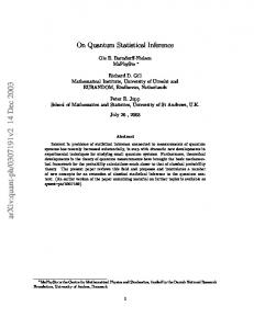
D5. Statistical Significance for Time Series Correlations SUMMARY: Statistically, the most important thing to know about time series is that the events are dependent. Thus any sufficient condition for statistical significance involving independent events is not appropriate for time-series events. For some great examples, visit the Spurious Correlation website, www.tylervigen.com: the source for the next figure. Figure 9: Correlation between Japanese US Car Sales and Motor-Vehicle Suicides
Ramsey and Schafer (2002, page 442) use the sample first-serial coefficient (r1) to adjust the independent standard error. SE(Average-Y) = Sqrt[(1+r1)/(1-r1)] [s/Sqrt(n)] Mu [ (Yi – v) | past history] = R*(Yi-1 – v) R is the population first serial correlation coefficient in the population. R is estimated by r1: the first serial correlation coefficient in the sample. The presence of temporal correlation will inflate the expected standard error. It may be that the inverse of this inflator could be used to deflate serial correlations and allow usage of the statistical significance shortcut for independent correlations.
3046