Dec 19, 2013 - Abstract. In Electrical Impedance Tomography (EIT), the internal conductivity of a body is recovered via current and voltage measure-.
A DATA-DRIVEN EDGE-PRESERVING D-BAR METHOD FOR ELECTRICAL IMPEDANCE TOMOGRAPHY
arXiv:1312.5523v1 [math.NA] 19 Dec 2013
S. J. HAMILTON, A. HAUPTMANN, AND S. SILTANEN Abstract. In Electrical Impedance Tomography (EIT), the internal conductivity of a body is recovered via current and voltage measurements taken at its surface. The reconstruction task is a highly ill-posed nonlinear inverse problem, which is very sensitive to noise, and requires the use of regularized solution methods, of which D-bar is the only proven method. The resulting EIT images have low spatial resolution due to smoothing caused by low-pass filtered regularization. In many applications, such as medical imaging, it is known a priori that the target contains sharp features such as organ boundaries, as well as approximate ranges for realistic conductivity values. In this paper, we use this information in a new edge-preserving EIT algorithm, based on the original D-bar method coupled with a deblurring flow stopped at a minimal data discrepancy. The method makes heavy use of a novel data fidelity term based on the so-called CGO sinogram. This nonlinear data step provides superior robustness over traditional EIT data formats such as current-to-voltage matrices or Dirichlet-to-Neumann operators.
1. Introduction Noise-robust solutions of ill-posed inverse problems are based on regularization strategies. For Electrical Impedance Tomography (EIT), the only proven regularization strategy is the low-pass filtered D-bar Method, which sets high scattering frequencies to zero resulting in smoothed images where sharp features important to applications such as medical imaging are absent. In this paper, we propose to recover edges in the smoothed EIT reconstructions by applying a deblurring flow stopped at a minimal data discrepancy (Figure 1), guided by a novel data fidelity term based on the so-called CGO sinogram, which provides superior robustness. Electrical Impedance Tomography (EIT) is an imaging modality where an unknown physical body is probed with electricity using electrodes attached to the surface of the body. The goal is to recover the internal conductivity distribution of the body based on current-to-voltage boundary measurements. EIT has applications in medical imaging, underground contaminant detection and industrial process monitoring. See [10] and [30, Chapter 12] for more details and applications of EIT. We formulate the inverse conductivity problem [8] for two-dimensional EIT in terms of voltage-to-current measurements. Let Ω ⊂ R2 be the unit disc. We model the conductivity by a bounded measurable function σ : Ω → R satisfying C > σ(z) ≥ c > 0 for almost every z ∈ Ω. For a prescribed boundary voltage f ∈ H 1/2 (∂Ω), the voltage potential u satisfies Date: December 19, 2013. 1
2
S. J. HAMILTON, A. HAUPTMANN, AND S. SILTANEN
True
D-bar
Improved
Figure 1. Left: true conductivity. Middle: blurry D-bar reconstruction from noisy EIT measurements, relative l1 error 15.11%. Right: reconstruction by the proposed edgepreserving algorithm, relative l1 -error 12.57%. the conductivity equation (1.1)
∇ · σ∇u = 0, u|∂Ω = f,
in Ω, on ∂Ω .
Infinite-precision voltage and current measurements are modeled by the Dirichlet-to-Neumann (DN), or voltage-to-current density, map ∂u (1.2) Λσ : f 7→ σ , ∂ν ∂Ω
where ν denotes the outward facing unit normal to ∂Ω. The goal of EIT is to recover the conductivity distribution σ(z) for z ∈ Ω, approximately, from the knowledge of a practical data matrix Λδσ satisfying kΛσ − Λδσ kY ≤ δ with known noise amplitude δ and an appropriate data space Y . EIT is a severely ill-posed inverse problem, in fact it is only log stable. By this we mean that small changes in boundary measurements can correspond to large changes in the internal conductivity distribution, and furthermore that noise in the data is amplified exponentially. Therefore, regularization is needed for the noise-robust recovery of σ from Λδσ . The forward map σ 7→ Λσ is too nonlinear to be covered by the presently available theory of iterative (Tikhonov-type) regularization. So far the only methodology providing proven regularization properties is the so-called D-bar method in dimension two [37, 29, 27]. Regularization for the 3D case is in progress, based on [11, 6, 14].1 There exists a nonlinear Fourier transform t : C → C that is intimately connected to EIT. Namely, Nachman showed in [33] that one can use infiniteprecision EIT data Λσ to completely determine t, and then apply the inverse transform, via solving a ∂ equation in the scattering variable, to recover the conductivity. However, in practice one never has such infinite-precision noise-free data; instead one works with noisy data Λδσ . The basic structure of the regularized D-bar method is shown in Figure 2. Practical data Λδσ only allow stable computation of the nonlinear Fourier transform in a disc centered at the origin in the frequency domain. One can then use the good part of the transform in the inversion, corresponding to a nonlinear low-pass 1Personal communication with Kim Knudsen and his team.
A DATA-DRIVEN EDGE PRESERVING D-BAR METHOD FOR EIT
3
(a) (b) Lowpass
filter
Inverse transform
Λδσ
Frequency domain Inverse transform
� ��
1 � �� � � ��
6 ?
(c)
Image domain
(d)
?
(e)
Figure 2. Schematic illustration of the nonlinear low-pass filtering approach to regularized 2D EIT. The simulated heart-and-lungs phantom (c) gives rise to a finite voltageto-current matrix Λδσ (orange square), which can be used to determine the nonlinear Fourier transform (a). Measurement noise causes numerical instabilities in the transform (see the irregular white patches in (a)), leading to an unstable and inaccurate reconstruction (d). However, multiplying the transform by the characteristic function of the disc |k| < R yields a lowpass-filtered transform (b), which in turn gives a noiserobust approximate reconstruction (e). filtering. The cut-off frequency R of the nonlinear low-pass filter depends logarithmically on the noise amplitude, tending to infinity asymptotically in the zero-noise limit. Analogously to linear low-pass filtering, the resulting image is smoothed and appears blurred. In general, noise-robust solutions of ill-posed inverse problems are based on complementing indirect and unstable measurement data with a priori information. The transform domain of the D-bar method organizes the measurement information neatly into a stable part (|k| < R) and unknown/unstable part (|k| ≥ R). Roughly speaking, information about the high frequencies of the unknown conductivity are missing from EIT data. What kind of a priori information do we have? In many applications of EIT it is reasonable to assume that the conductivity is piecewise constant with crisp boundaries between the homogeneous regions. Those boundaries have significant high-frequency content which is not stably represented in the data. Modern imaging science provides several options for sharpening blurred images, which may help to recover the edges in the true conductivity. The most straightforward edge-sharpening approach, the Perona-Malik
4
S. J. HAMILTON, A. HAUPTMANN, AND S. SILTANEN
Iteration number
0
15
30
45
60
75
20.3
17.76
17.41
17.28
17.36
17.56
Segmentation by AT flow Enhanced contrast Error in CGO sinogram (%)
Figure 3. Graphical overview of the proposed EIT reconstruction algorithm. The starting point of the AmbrosioTortorelli segmentation flow is the outcome of the low-pass filtered D-bar method (iteration 0). The final reconstruction is chosen to be the contrast-enhanced image having the smallest CGO sinogram error. The measured EIT data is used in the calculation of the error. anisotropic diffusion approach [34] (see [36, 39] for its generalizations) proved insufficient due to either too smooth edges or instability at high gradients. However, the technique that proposed by Ambrosio and Tortorelli [2] as an approximation to the classical Mumford-Shah image segmentation functional [31] worked excellently. Areas separate nicely and develop constant values, while the gradient can be controlled by the auxiliary variable of the model. This functional has been widely used in image processing, see for instance [9, 15, 25]. On the other hand the approach is rather uncommon for inverse problems, there are a few examples in signal restoration [22] and particular for EIT imaging [35]. It is well-known that minimizing the Ambrosio-Tortorelli (AT) functional can be used to sharpen and segment blurry images [2, 36]. The image flows in time according to a nonlinearly deforming diffusivity. High gradients in the initial image will develop sharp edges, while slowly varying regions will tend to constant-value areas in the final image. See Section 3 for more information about AT. Simply minimizing the AT functional for the blurry D-bar reconstruction will introduce edges, but we need to ensure that the change is for the better. In particular in medical imaging applications we need to avoid introducing artefacts. We propose controlling the AT flow using the measured EIT data. How should one check the compatibility of the evolving conductivity to the measured data? One option would be to simulate the EIT measurement matrix Λt at each time step for the evolving AT image and ensure that the distance to the measured matrix Λδσ decreases. However, more robust control is provided by a novel concept called CGO sinogram. It consists of the traces of the complex geometric optics (CGO) solutions (of the D-bar method) at the boundary, corresponding to low-frequency spectral parameters only. The
A DATA-DRIVEN EDGE PRESERVING D-BAR METHOD FOR EIT
5
CGO sinogram is stable to compute from EIT data and contains geometric information about the conductivity in a far more explicit form than the DN map (see Figure 4). While the AT flow will introduce edges, as desired, it also lowers the contrast in the image. To overcome this problem, we introduce a contrastenhancement step. See Figure 3 for the result. We remark that our method provides a novel connection between the PDE-based inverse problems community and the PDE-based image processing community having a potentially strong impact on both. The remainder of the paper is organized as follows. Sections 2-4 contain the theory behind the key pieces in the new edge preserving reconstruction method guided by the data-driven contrast enhancement of Section 5. In Section 2, the D-bar method is reviewed. The Ambrosio-Tortorelli functional used for the recovering edges is described in Section 3. In Section 4, the novel CGO sinogram is introduced and the data-driven contrast enhancement is presented in Section 5. For the reader’s convenience, Section 6 is dedicated to an explicit description of the algorithm. In Section 7 the proposed algorithm is demonstrated on simulated noisy EIT measurements. A discussion of the results is given in Section 8 and the take home message and conclusions of the paper are given in Section 9. 2. A Brief Review of the D-bar Method By the D-bar method we refer to the EIT algorithm based on the theory introduced in [33], first implemented in [37] and equipped with an explicit regularization step in [27]. Alternative D-bar methods have since emerged which handle complex coefficients [18, 19, 20], less regular conductivities [7, 26, 28] and merely bounded L∞ conductivities [4, 5, 3]. However, for the purpose of this article, with future partial data approaches in mind we proceed with the well-established setting of [27], the only 2D approach with a proven regularization strategy. The core idea in the D-bar method is to use a nonlinear Fourier transform tailor-made for EIT. To define the transform we need modified exponential functions, also called Complex Geometrical Optics (CGO) solutions. Assume (for now) that σ ∈ C 2 (Ω) and that σ = 1 in a neighborhood of the boundary. The conductivity equation (1.1) can then be transformed, √ using the change of variables ψ = σu, to the Schr¨odinger equation [−∆ + q]ψ = 0. Here we define the potential q by extending σ from Ω to all of C by setting σ(z) ≡ 1 for z ∈ C \ Ω and writing p ∆ σ(z) q(z) = p . σ(z) Note that q has compact support in Ω. We introduce an auxiliary variable k ∈ C\{0} and look for CGO solutions ψ(z, k) satisfying (2.1)
[−∆ + q(·)]ψ(·, k) = 0
6
S. J. HAMILTON, A. HAUPTMANN, AND S. SILTANEN
with the asymptotic condition e−ikz ψ(z, k) − 1 ∈ W 1,p (R2 ). We associate R2 with C by the mapping z = (x, y) 7→ x + iy, so that kz = (k1 + ik2 )(x + iy) denotes complex multiplication. CGO solutions were originally introduced by Faddeev in [16] and later reinvented in the context of inverse problems in [38]. By [33] we know that the solutions ψ exist and are unique for any 2 < p < ∞ for the potentials we consider here. (Other kinds of potentials may have exceptional points, or k values with no unique ψ( · , k). See [32] for more details.) The regularized D-bar reconstruction algorithm is comprised of the following steps: 1
2
Λδσ −→ tR (k) −→ σ R (z). Step 1: From boundary measurements Λδσ to scattering data tR . For each fixed k ∈ C \ 0, solve the Fredholm integral equation of the second kind for z ∈ ∂Ω Z h i Gk (z − ζ) Λδσ − Λσ ψ δ (ζ, k) dS(ζ), (2.2) ψ δ (z, k) = eikz − ∂Ω
where Gk is the Faddeev Green’s function [16], with asymptotics matching ψ, defined by Z eiz·ξ 1 ikz dξ. Gk (z) := e gk (z), gk (z) := (2π)2 R2 |ξ|2 + 2k (ξ1 + iξ2 )
(2.3)
Evaluate the scattering transform tR using the boundary traces ψ δ from (2.2) (R � ¯ � eik¯z Λδσ − Λσ ψ δ (z, k) dS(z), |k| < R R ∂Ω t (k) := 0 |k| ≥ R.
Step 2: From scattering data tR to conductivity σ R . Fix z ∈ Ω and solve the ∂ k equation 1 R (2.4) ∂ k µR (z, k) = t (k)e(z, −k)µR (z, k), 4π k¯ � � ¯z , saving µ(z, 0). The regularized where e(z, k) := exp i kz + k¯ conductivity σ R is recovered by �2 (2.5) σ R (z) = µR (z, 0) . If σ 6= 1 near ∂Ω, but is instead a constant σ0 , the entire problem can be scaled as follows. Let σ ˜ = σ/σ0 denote a scaled conductivity which then has a value of 1 near ∂Ω. The corresponding scaled DN map is then computed by Λσ˜ = σ0 Λσ . R After recovering σ ˜ from Step 2 of the D-bar algorithm above, undo the scaling by multiplying by σ0 yielding the correct σ R .
A DATA-DRIVEN EDGE PRESERVING D-BAR METHOD FOR EIT
7
The algorithm described above has been used successfully on both simulated and experimental data [37, 29, 23, 27]. In many applications it is well known that high frequency features such as jump discontinuities and clear edges are present, e.g. organ boundaries. However, the lowfrequency truncation needed in the regularized D-bar algorithm results in smoothed/blurred reconstructions where these high-frequency features are often absent. This calls for post-processing of the D-bar reconstruction to reintroduce the missing features. We propose minimizing a functional in a process known as Ambrosio-Tortorelli image segmentation. 3. Diffusive Image Segmentation Consider the following image processing problem. We begin with a smooth image u e, which is the result of a blurring process applied to a clean, piecewise constant image u. How can we recover u from u e? In 1985, Mumford and Shah introduced the following functional for the purpose of detecting boundaries in general images [31]: Z Z 2 (3.1) EM S (u, K) = |∇u| dx + β (u − u e)2 dx + α|K|, Ω\K
Ω
where K denotes a curve segmenting Ω, |K| the length of K, and the two parameters α, β > 0 are used for weighting the terms. The idea is to find the minimum of EM S (u, K) over images u and curves K; the minimizing image is then considered an edge-preserving reconstruction of u from u e. As K is unknown and singular, numerically minimizing (3.1) is a challenging task; in particular formulating a gradient-descent method with respect to K is not straightforward. Therefore, Ambrosio and Tortorelli [2] proposed an elliptic approximation to (3.1) by introducing an edge-strength function v : Ω → [0, 1] for controlling the gradient of u. The Ambrosio-Tortorelli (AT) functional is defined by � � Z (1 − v)2 2 2 2 2 dx. (3.2) EAT (u, v) = β(u − u e) + v |∇u| + α ρ|∇v| + 4ρ Ω The additional parameter ρ > 0 specifies, roughly speaking, the edge width of u. Then EAT Γ-converges to EM S as ρ → 0 [2], which can be understood as solutions of (3.2) converge to solutions of (3.1) with the parameter ρ → 0, for further explanations see [9]. The advantage of (3.2) over (3.1) is that the minimizer can be obtained by an artificial time evolution formulated via a coupled PDE as the gradientdescent equations with an imposed homogeneous Neumann boundary condition: ∂t u = div(v 2 ∇u) + β(u − u e) in Ω × (0, T ], v|∇u|2 1 − v ∂t v = ρ∆v − + in Ω × (0, T ], (3.3) α 4ρ ∂n u = 0, ∂n v = 0 on ∂Ω × (0, T ], u(·, 0) = u e, v(·, 0) = v0 in Ω. The equations in (3.3) are referred to as the AT flow. With these gradient descent equations, implementing the numerical minimization algorithm is
8
S. J. HAMILTON, A. HAUPTMANN, AND S. SILTANEN
now a straightforward task (use finite differences or a parabolic finite element solver). Numerous modifications of the functionals (3.1) and (3.2) have been proposed, e.g. substituting the squared norm |∇u|2 with |∇u| in the spirit of Total Variation [1], or adjusting the auxiliary function v as in [15]. The effect of (3.2) can be visualized as follows. First, keeping v fixed, one sees that the first equation (3.3) minimizes the functional Z β(u − u e)2 + v 2 |∇u|2 dx = βku − u ek2L2 (Ω) + kv|∇u|k2L2 (Ω) . (3.4) Ω
The representation on the right hand side is a typical form for stating regularization problems. The first fidelity term controls the distance of the obtained solution from the initial reconstruction, whereas the regularization term weights ∇u with respect to the positive (here fixed) edge-strength function v. The balance between the fidelity and regularization terms can be controlled by the regularization parameter β > 0. In the same manner, keeping u fixed, from the second equation in (3.3), we have a minimizer for a functional that can be written as !2 Z 4ρ 2 1 + |∇u| 1 α (3.5) 4ρ|∇v|2 + − v dx. 2 ρ 1 + 4ρ Ω α |∇u| Here we clearly see the auxiliary variable can be interpreted as a smooth approximation to the Perona-Malik filter [34], given by 1 (3.6) g(|∇u|2 ) = . 4ρ 1 + α |∇u|2 To state a minimizing algorithm on the equations (3.3), one needs to specify an initial guess of v0 . This is where the interpretation (3.6) comes in handy and we can set the first approximation for the auxiliary variable as v0 = g(|∇e u|2 ). Perona and Malik based their edge-aware smoothing on the diffusion equation (3.7)
∂t u = div(g(|∇u|2 )∇u).
Historically, the model in (3.7) has a strong effect on noise removal and the smoothing of images, by keeping edges stable for a long time in the process. However, one downside of this particular diffusion concept is that the limiting function is a constant and hence a stopping criterion during the iteration is needed [39]. In contrast, the AT functional in (3.2) converges to the Mumford-Shah segmentation functional (3.1), for which minimizers are known to be piecewise constant with respect to the discontinuity set K [13]. By using the AT functional instead, the problem of defining a proper stopping criterion is shifted to choosing the correct parameters α and β, and making it possible to adapt the minimization problem to the reconstruction task at hand. 4. The CGO Sinogram The central idea of this study is to complement the regularized D-bar method by applying an edge-introducing image processing algorithm to a blurred EIT reconstruction. However, when manipulating the EIT image we need to
A DATA-DRIVEN EDGE PRESERVING D-BAR METHOD FOR EIT
9
ensure that we are improving the image. This is accomplished by monitoring the resulting error in a novel way (see Figure 3). The obvious approach is to monitor the data discrepancy kΛδσ − Λσ0 kY , where Λδσ is the measured data and σ 0 denotes the enhanced reconstruction, but the basic observation behind our new data fidelity term is that the DN map encodes geometric information nonlinearly in a very complicated, non-intuitive, and unstable way. For example, take a look at the three conductivities shown in the left column of Figure 4. They each have one circular inclusion of conductivity two embedded into a homogeneous background of unit conductivity. The middle column shows the matrix approximations to the DN map. Can you deduce the location of the inclusion from the DN map? We didn’t think so. Now take a look at the right column in Figure 4. There we show the absolute value of the difference of the CGO solution µ(z, k) = µ(eiθ , 2eiϕ ) and its limiting value 1, as a function of the spectral frequency angles ϕ (vertical axis) and physical angles θ (horizontal axis) where both angles range from 0 to 2π. The locations of the inclusions are immediately discernible! Clearly, Figure 4 is just one very simple example. See Figure 5 for a more complicated situation, where we add a circular inclusion to a heartand-lungs phantom. The location of the inclusion is clearly indicated in the difference of the two CGO sinograms. We believe that the numerical evidence presented in Figures 4 and 5 reflects a more general fact: calculating the CGO sinogram (4.1)
Sσ (θ, ϕ, r) := µ(eiθ , reiϕ ) − 1
from the EIT measurements is stable (for r > 0 inside the region of proven stability) and encodes the geometry of the conductivity in a useful and more transparent way.
10
S. J. HAMILTON, A. HAUPTMANN, AND S. SILTANEN
Conductivity
DN matrix
CGO sinogram
3π/2
3π/2
π
π π/2
arg(k)
0 π/2
2π arg(z)
Figure 4. Left: conductivities with background one and circular inclusion of conductivity two. The polar coordinate angle of the center of the inclusion is indicated. Middle: the matrix approximation to the Dirichlet-to-Neumann map corresponding to each conductivity. More precisely, the matrix approximation to Λδσ − Λ1 is plotted to remove the dominating diagonal elements and bring out the differences between a homogeneous and inhomogeneous conductivity, σ1 and σ, more clearly. Right: CGO sinogram corresponding to each conductivity. The color shows the values of |µ(z, k) − 1| for |z| = 1 and |k| = 2. Note that the CGO sinograms carry clear geometric information, as opposed to the DN maps.
A DATA-DRIVEN EDGE PRESERVING D-BAR METHOD FOR EIT
Conductivity 1
Conductivity 2
11
Difference
5π 4
5π 4
CGO sinogram 1
CGO sinogram 2
Difference
0
2π 5π 4
Figure 5. Top row: two heart-and-lungs conductivities (one with an extra circular inclusion), and their difference. The conductivity values are as follows. Heart: 4 (red), lungs: 1/2 (blue), background: 1 (green) and inclusion: 2 (orange). The polar coordinate angle of the center of the inclusion is indicated. Bottom row: absolute values of the corresponding CGO sinograms and their absolute difference. Note that the location of the inclusion is clearly visible in the bottom right plot.
12
S. J. HAMILTON, A. HAUPTMANN, AND S. SILTANEN
5. Contrast Enhancement The Ambrosio-Tortorelli (AT) segmentation flow, discussed in Section 3 above, can transform a blurry image into a sharper image. However, the AT flow comes with a reduction in contrast, which in turn is a key benefit of EIT imaging. To overcome this obstacle, we propose using a data-driven contrast enhancement technique kept in check by the CGO sinogram. Let f (z) := σ AT (z) − 1, denote the difference between the conductivity after AT flow and the constant 1 (the value near the boundary). Recall the a priori constants c and C known to bound the conductivity 0 < c < σ(z) < C. In practice, such ballpark bounds are readily available. For example, in chest imaging, using an applied current with frequency 100 kHz, internal conductivites range from around 0.02 Siemens/meter (e.g. fat) to 0.71 Siemens/meter (e.g. heart tissue) [12]. Denote by m and M the following minimum and maximum values m := minf (z), z∈Ω
For (s, t) ∈ (5.1)
M := maxf (z). z∈Ω
[0, 1]2
define ( (z) (c − 1) s fm fs,t (z) = f (z) t M (C − 1)
for z satisfying f (z) < 0 for z satisfying f (z) ≥ 0
and set (5.2)
σs,t (z) := 1 + fs,t (z).
The optimal contrast enhanced conductivity σ CE is determined by minimizing the CGO sinogram error over (s, t) ∈ [0, 1]2 ( ) (5.3)
(s0 , t0 ) := arg min (s,t)∈[0,1]2
kSδσ (θ, ϕ, R) − Sσs,t (θ, ϕ, R)k2L2 (T2 )
,
and using (5.2) to define (5.4)
σ CE (z) := σs0 ,t0 (z).
Various algorithms are available to find an approximation to the optimal s0 and t0 in (5.3). In this work we apply a derivative free pattern search algorithm which is known to be stable in the presence of noise: the DIRECT (DIviding RECTangles) pattern search for global optimization [24, 17]. In Figure 6 we see clear evidence that minimizing with respect to the CGO sinogram is advantageous to the DN map for preserving important image features. The figure shows the heart and lungs test problem with conductivity reconstructed by the D-bar algorithm (left) and the optimal contrast-enhanced images chosen by minimizing the error of CGO sinogram (middle) and DN map (right) to the measured data. Clearly, the image chosen by the CGO sinogram minimization more accurately portrays the original than the one chosen by the DN map. Even though both solutions were able to minimize the l1 -error to the true phantom, from the introductory example in Figure 1, the features preserved differ immensely (i.e. the heart is barely visible in the DN guided minimization).
A DATA-DRIVEN EDGE PRESERVING D-BAR METHOD FOR EIT
D-bar
Error 15.11%
CGO
Error 14.72%
13
DN
Error 15.05%
Figure 6. Comparison of contrast enhanced solutions. Left: initial D-bar reconstruction with relative l1 -error 15.11% to the original phantom. Middle: solution chosen by minimal CGO sinogram error, relative l1 -error 14.72% to the original phantom. Right: solution with minimal error in DN maps, relative l1 -error 15.05% to the original phantom. 6. A Data-Driven Edge-Preserving D-bar Algorithm The aim of this paper is to combine the strengths of each the methods described above in Sections 2-4 with the data-driven contrast enhancement of Section 5. We compute the reconstruction of the conductivity with the regularized D-bar method and reintroduce edges by a data-driven postprocessing of the image. The post-processing is monitored by the CGO sinogram error which incorporates geometric information about the reconstruction. We propose the following Data-Driven Edge-Preserving D-bar Algorithm: Step 1: Fix R > 0 and compute the regularized D-bar reconstruction σ R using the D-bar algorithm described in Section 2. Step 2: Fix a radius r located in the stable disc: R > r > 0. (i) Compute the CGO sinogram Sδσ (θ, ϕ, r) from the original noisy data Λδσ by solving the boundary integral equation (2.2) for ψ δ (z, k) and setting Sδσ (θ, ϕ, r) := exp(−irei(ϕ+θ) ) ψ δ (eiθ , reiϕ ) − 1. (ii) Calculate the CGO sinogram SδσR (θ, ϕ, r) for the D-bar image. (iii) Record the relative CGO sinogram error E0 :=
kSδσ (θ, ϕ, R) − SσR (θ, ϕ, R)kL2 (T2 ) . kSδσ (θ, ϕ, R)kL2 (T2 )
Step 3: Reintroduce edges to σ R via minimization of the Ambrosio-Tortorelli functional by solving the gradient descent equations (3.3). (i) Initialize the constants β, α and ρ. (ii) Calculate the initial approximation for the auxiliary function as v0 = g(|∇σ R |2 ) defined by (3.6).
14
S. J. HAMILTON, A. HAUPTMANN, AND S. SILTANEN
(iii) Choose a time step t and begin solving (3.3) iteratively. Step 4: Check the flow every J, e.g. J = 5, time steps as follows. For the j-th check: (i) Denote the image to be checked σjAT . (ii) Determine σjCE , the optimal contrast enhanced version of σjAT using the CGO sinogram optimization method described in Section 5. (iii) Record the CGO sinogram error Ej for σjCE . (iv) If Ej < Ej−1 , return to the AT flow with σjAT (the non-contrast enhanced version) and repeat steps (i)-(iii). If not, or if a maximum number of iterations Jmax is reached, set (6.1)
σN EW (z) := σjCE (z) and the algorithm is complete. 7. Computational results
We tested the algorithm on simulated noisy EIT measurement data for two test cases, of potential interest for the medical and industrial communities, respectively. To simulate the EIT measurements, we solved the Neumann problem corresponding to the conductivity equation (7.1)
∇ · σ∇u = 0, z ∈ Ω ⊂ R2 z ∈ ∂Ω σ ∂u ∂ν = gj ,
for j = −16, . . . , −1, 1, . . . , 16, representing 32 linearly independent current patterns. In this paper Ω is the unit disc, and we used the Fourier basis functions � � 1 gj eiθ = √ eijθ , z = eiθ ∈ ∂Ω . 2 The matrix approximation to the DN maps Λσ and Λ1 (the DN corresponding to a uniform unit conductivity) were computed for each test problem using the standard methods described in [30]. The numerical implementation of the regularized D-bar method was first fully described in [27] and later explained in more detail in [30, Section 13.2], including freely available Matlab code. A discussion of a numerical implementation with finite differences of the AT flow can be found in [15]. In this study, we used the Matlab integrated PDE solver for the equations (3.3) and for each test problem below the choice of regularization parameters is given. Additional zero-mean random Gaussian noise was added to the DN matrix Λσ so that (7.2)
kΛσ − Λδσ kH 1/2 (∂Ω)→H −1/2 (∂Ω) ≤ δ
using the methods described in [27]. While types of noise and their magnitudes vary among EIT devices, a benchmark of around 0.01% has been obtained [10]. The resulting CGO sinogram and conductivity errors stated below are given as relative errors. The relative error of CGO sinograms corresponding
A DATA-DRIVEN EDGE PRESERVING D-BAR METHOD FOR EIT
15
to the original conductivity σ and to some reconstruction σd was measured by (7.3)
kSδσ (θ, ϕ, R) − Sσd (θ, ϕ, R)kL2 (T2 ) . kSδσ (θ, ϕ, R)kL2 (T2 )
Similarly we measured the relative error of the reconstructed conductivities to the original via kσ − σd kLp (Ω) (7.4) kσkLp (Ω) with p = 1 or p = 2. 7.1. A Heart-and-Lungs Phantom. The leftmost image in Figure 7 shows our piecewise constant phantom. The lungs have conductivity 0.5, the heart has conductivity 2, and the background has unit conductivity. The D-bar reconstruction was obtained using a truncation radius of R = 4 in the scattering data. The D-bar method allows computing the reconstruction at arbitrary points in the z-plane, and we chose to reconstruct directly at the points of the FEM mesh (of 33025 elements) to be used in the AT flow. Note that the FEM mesh for the AT flow is different from the FEM mesh of the forward conductivity solver used to compute the DN map Λσ . We have added additional noise of amplitude δ = 0.005 to the DN map satisfying (7.2), and corresponding to 0.5% noise far surpassing the 0.01% measurement. The D-bar reconstruction is shown in the middle image in Figure 7); it has a relative CGO sinogram error of 20.3%. The AT flow (Step 3) was computed with parameters α = 200, β = 0.1, ρ = 0.1, and the contrast enhanced solution σ CE was computed every fifth iteration using the CGO sinogram with |k| = 2, well within the reliable region for the regularized D-bar method. The boundary constants were roughly chosen as c = 0.1 and C = 4. A summary of the obtained solutions is illustrated in Figure 8. The optimal solution was obtained at iteration 45 with a relative error in CGO sinogram of 17.28%. Figure 9 displays the error in CGO sinogram as well as the error of reconstruction to the true conductivity throughout the evolution of the AT flow.
16
S. J. HAMILTON, A. HAUPTMANN, AND S. SILTANEN
True conductivity
D-bar
Improved
Figure 7. Illustration of original Heart-and-Lungs phantom with the initial D-bar reconstruction (truncation radius R = 4) and the contrast-enhanced diffused solution of the Ambrosio-Tortorelli functional at iteration 45.
Iteration 30
Iteration 45
CE solutions
AT flow
Iteration 15
Figure 8. Illustration of the minimization process of the Ambrosio-Tortorelli functional for three different stages, including the contrast enhanced solutions with smallest error in CGO sinogram.
7.2. An Industrial Pipe Phantom. The second test case is an example from the oil industry. It roughly models a pipe with oil (top layer, conductivity 1.2), water (middle layer, conductivity 2.0), and sand (bottom layer, conductivity 0.3) similar to the test problem of [3]. The initial D-bar reconstruction is computed on the same mesh with a truncation radius of R = 6 and additional noise of 0.01% in the measured DN map. The parameters for the AT flow and contrast enhancement were chosen the same as in the previous example. The CGO sinograms were computed with a small radius of |k| = 0.5 far within the reliable region.
A DATA-DRIVEN EDGE PRESERVING D-BAR METHOD FOR EIT
rel. l2 -error of CGO sinogram
17
rel. l1 -error of reconstructed conductivity 0.155 AT flow CE solutions
AT flow CE solutions
0.15 0.3
0.275
0.145
0.25
0.14
0.225
0.135
0.13
0.2
0.125 0.175
0
10
20
30
40
50
60
70
80
90
100
0.12
0
10
20
30
40
50
60
70
80
90
Number of iterations
Figure 9. Convergence plot of the AT minimized solutions CGO sinograms in relative l2 -error to the true measurement (Left) and the relative l1 -error of the reconstructions to the true Heart-and-Lungs conductivity (Right). The minimization of the CGO sinogram error with the proposed algorithm did not converge and hence the algorithm stopped at the maximum number of iterations chosen as Jmax = 200. The error in the CGO sinogram has been halved from 17.53% in the original D-bar reconstruction, to 8.73% in the improved reconstruction obtained with the new algorithm (left plot of Figure 11). The right plot shows the error in the contrast enhanced versions of conductivities after the AT flow. Their error increased, after an initial decrease, from 15.09% of the D-bar reconstruction to 15.32% of the reconstruction obtained by the AT flow after 200 iterations and 18.35% of the corresponding contrast enhanced solution. However, we point out that in practice such a comparison (right plot of Figure 11) is not possible as the true conductivity is unknown, and only the left plot is possible, where in fact we see a clear decrease in the CGO error. 8. Discussion The heart-and-lungs phantom of Section 7.1 is of particular interest, since it represents, an admittedly simplified version of, a major application of electrical impedance tomography in the medical field: monitoring the blood and air flow in a patient’s heart and lungs. With the proposed algorithm we were able to clearly distinguish the left and right lung as well as introduce clear edges, see Figure 7. As discussed above, a level of 0.5% noise is reasonably high for EIT measurements and hence gives a good impression of how the algorithm behaves with noise corrupted data. The original D-bar recovered conductivity (see the middle image in Figure 7) has good contrast but lacks sharpness, as is typical for D-bar reconstructions. A summary of the AT flow is illustrated in Figure 8. Notice that the AT flow gradually divides the two lungs, and that the separated areas converge to constant values. As seen in the right plot of Figure 9, the AT flow (blue
100
18
S. J. HAMILTON, A. HAUPTMANN, AND S. SILTANEN
True conductivity
D-bar
AT iteration 200
Contrast enhanced
Figure 10. Illustration of original pipe phantom with the initial D-bar reconstruction (Truncation radius 6) in the top row. Reconstruction after 200 iterations of the AT flow (Bottom left) and the corresponding contrast enhanced solution (Bottom right).
rel. l2 -error of CGO sinogram
rel. l1 -error of reconstructed conductivity 0.2
0.45
AT flow CE solutions
AT flow CE solutions
0.19
0.4
0.18 0.35
0.17 0.3
0.16
0.15
0.25
0.14 0.2
0.13 0.15
0.12 0.1
0.05
0.11
0
20
40
60
80
100
120
140
160
180
200
0.1
0
20
40
60
80
100
120
140
Number of iterations
Figure 11. Convergence plot of the AT minimized solutions CGO sinograms in relative l2 -error to the true measurement (Left) and the relative l1 -error of the reconstructed pipe conductivity (Right).
160
180
200
A DATA-DRIVEN EDGE PRESERVING D-BAR METHOD FOR EIT
19
line) clearly minimizes the l1 -error of the evolved conductivity to the true conductivity. Furthermore, the behavior of its corresponding CGO sinogram error (blue plus sign markers in the left plot), initially decreasing but followed by a sharp increase, reinforces the need for a contrast enhancement step. Note that the CE solutions have a similar behavior in both CGO sinogram error and the reconstruction error of the conductivity, and that the CE evolved conductivities have smaller relative errors to the true conductivity than their non CE counterparts.
The second test case (Section 7.2) is an example from the oil industry. When measuring a pipe with oil (top layer), water (middle layer), and sand (bottom layer) one wants to know how much oil is transported in the pipe, making it important to distinguish the levels of each substance clearly, i.e. their edges. The new reconstruction has clear and sharp edges dividing the different substances and one can tell easily how much of each substance is present in the pipe. As one can see in Figure 10, the structure of the pipe has been reintroduced to the reconstruction, delivering a realistic view of the imaged target. The right plot in Figure 11 shows that the error in reconstructed conductivities did not decrease as nicely as in the Heart-and-Lungs phantom. In fact, the reconstruction error increased from 15.09% of the D-bar reconstruction to 18.35% of the contrast enhanced solution of the last iteration 200 in the AT flow. A reason for the higher error can be seen in Figure 10, the contrast enhancement increases the conductivity of the top layer as well as the middle layer, which produces a higher error in the middle layer. This suggests that more sensitive models for the contrast enhancement may be needed. Nevertheless, the information contained in the contrast enhanced solution is far more useful for evaluation of the target and suggests that the CGO sinogram contains more information about the reconstructions geometry.
9. Conclusions A novel edge-preserving D-bar method with a data-driven contrast enhancement was introduced and tested on simulated EIT measurement data. The algorithm works as advertised by both sharpening and enhancing the contrast of the reconstruction, even in the presence of additional noise added to the Dirichlet-to-Neumann boundary measurements. Key to the approach is the invention of the CGO sinogram, a more reliable and geometrically transparent quantity than the DN map. While outside the scope of this paper, the authors are excited by the implications this work has for the partial data problem. As the traces of the CGO solutions are preserved for small |k| frequencies on the accessible portion of the boundary [21], the CGO sinogram provides an important breakthrough towards new uses of this nonlinear data. Our results also have implications outside the realm of D-bar methods. The traditional regularization approach for EIT reconstructions is to find
20
S. J. HAMILTON, A. HAUPTMANN, AND S. SILTANEN
the minimizer of a functional of the form (9.1)
kΛδσ − Λσ0 kY + αkσ 0 kX ,
where the X norm corresponds, for instance, to Tikhonov or Total Variation regularization, and 0 < α < ∞ is a regularization parameter. Replacing the traditional data fidelity term in (9.1) by an analogous term based on the CGO sinogram leads to the functional (9.2)
kSσ (θ, ϕ, r) − Sσ0 (θ, ϕ, r)k2L2 (T2 ) + αkσ 0 kX ,
where T2 denotes the two-dimensional torus. Based on the evidence seen in Figures 4 and 5, we strongly suspect that using (9.2) would lead to superior reconstructions compared to (9.1). A similar comment applies to the likelihood distributions used in Bayesian inversion approaches for EIT. Acknowledgments The study was supported by the SalWe Research Program for Mind and Body (Tekes - the Finnish Funding Agency for Technology and Innovation grant 1104/10) and by the Academy of Finland (Finnish Centre of Excellence in Inverse Problems Research 2012–2017, decision number 250215). References [1] R. Alicandro, A. Braides, and J. Shah, Approximation of non-convex functionals in GBV, 1998. [2] L. Ambrosio and V. M. Tortorelli, Approximation of functionals depending on jumps by elliptic functionals via Γ-convergence, Communications on Pure and Applied Mathematics, 43 (1990), pp. 999–1036. ¨ iva ¨ rinta, A. Pera ¨ ma ¨ ki, and S. Siltanen, Direct [3] K. Astala, J. Mueller, L. Pa electrical impedance tomography for nonsmooth conductivities, Inverse Problems and Imaging, 5 (2011), pp. 531–549. ¨ iva ¨ rinta, A boundary integral equation for Calder´ [4] K. Astala and L. Pa on’s inverse conductivity problem, in Proc. 7th Internat. Conference on Harmonic Analysis, Collectanea Mathematica, 2006. ¨ iva ¨ rinta, Calder´ [5] K. Astala and L. Pa on’s inverse conductivity problem in the plane, Annals of Mathematics, 163 (2006), pp. 265–299. [6] J. Bikowski, K. Knudsen, and J. L. Mueller, Direct numerical reconstruction of conductivities in three dimensions using scattering transforms, Inverse Problems, 27 (2011). [7] R. M. Brown, Global uniqueness in the impedance imaging problem for less regular conductivities, SIAM Journal on Mathematical Analysis, 27 (1996), pp. 1049–1056. ´ n, On an inverse boundary value problem, in Seminar on Numerical [8] A.-P. Caldero Analysis and its Applications to Continuum Physics (Rio de Janeiro, 1980), Soc. Brasil. Mat., Rio de Janeiro, 1980, pp. 65–73. [9] A. Chambolle, Image segmentation by variational methods: Mumford and shah functional and the discrete approximations, SIAM Journal on Applied Mathematics, 55 (1995), pp. 827–863. [10] M. Cheney, D. Isaacson, and J. C. Newell, Electrical impedance tomography, SIAM Review, 41 (1999), pp. 85–101. [11] H. Cornean, K. Knudsen, and S. Siltanen, Towards a d-bar reconstruction method for three-dimensional eit , Journal of Inverse and Ill-Posed Problems, 14 (2006), pp. 111–134. [12] I. N. R. Council, Dielectric properties of body tissues, 2013.
A DATA-DRIVEN EDGE PRESERVING D-BAR METHOD FOR EIT
21
[13] E. De Giorgi, M. Carriero, and A. Leaci, Existence theorem for a minimum problem with free discontinuity set, Archive for Rational Mechanics and Analysis, 108 (1989), pp. 195–218. [14] F. Delbary, P. C. Hansen, and K. Knudsen, Electrical impedance tomography: 3D reconstructions using scattering transforms, Applicable Analysis, 0 (0), pp. 1–19. [15] E. Erdem and S. Tari, Mumford-shah regularizer with contextual feedback, Journal of Mathematical Imaging and Vision, 33 (2009), pp. 67–84. [16] L. D. Faddeev, Increasing solutions of the Schr¨ odinger equation, Soviet Physics Doklady, 10 (1966), pp. 1033–1035. [17] D. E. Finkel, Direct optimization algorithm user guide, tech. report, Center for Research in Scientific Computation, North Carolina State University, 2003. [18] E. Francini, Recovering a complex coefficient in a planar domain from Dirichlet-toNeumann map, Inverse Problems, 16 (2000), pp. 107–119. [19] S. Hamilton, C. Herrera, J. L. Mueller, and A. VonHerrmann, A direct D-bar reconstruction algorithm for recovering a complex conductivity in 2-D, Inverse Problems, 28 (2012), p. 095005. [20] S. J. Hamilton and J. L. Mueller, Direct EIT reconstructions of complex admittivities on a chest-shaped domain in 2-D, IEEE Transactions on Medical Imaging, 32 (2013), pp. 757–769. [21] S. J. Hamilton and S. Siltanen, Nonlinear inversion from partial data EIT: Computational experiments, Contemporary Mathematics:(accepted), (2013). [22] T. Helin and M. Lassas, Hierarchical models in statistical inverse problems and the mumford–shah functional, Inverse problems, 27 (2011), p. 015008. [23] D. Isaacson, J. Mueller, J. Newell, and S. Siltanen, Imaging cardiac activity by the D-bar method for electrical impedance tomography, Physiological Measurement, 27 (2006), pp. S43–S50. [24] D. R. Jones, C. D. Perttunen, and B. E. Stuckman, Lipschitzian optimization without the lipschitz constant, Journal of Optimization Theory and Applications, 79 (1993), pp. 157–181. [25] M. Jung, X. Bresson, T. F. Chan, and L. A. Vese, Nonlocal Mumford-Shah regularizers for color image restoration, IEEE Trans. Image Process., 20 (2011), pp. 1583– 1598. [26] K. Knudsen, A new direct method for reconstructing isotropic conductivities in the plane, Physiological Measurement, 24 (2003), pp. 391–403. [27] K. Knudsen, M. Lassas, J. Mueller, and S. Siltanen, Regularized D-bar method for the inverse conductivity problem, Inverse Problems and Imaging, 3 (2009), pp. 599– 624. [28] K. Knudsen and A. Tamasan, Reconstruction of less regular conductivities in the plane, Communications in Partial Differential Equations, 29 (2004), pp. 361–381. [29] J. Mueller and S. Siltanen, Direct reconstructions of conductivities from boundary measurements, SIAM Journal on Scientific Computing, 24 (2003), pp. 1232–1266. [30] J. Mueller and S. Siltanen, Linear and Nonlinear Inverse Problems with Practical Applications, vol. 10 of Computational Science and Engineering, SIAM, 2012. [31] D. Mumford and J. Shah, Boundary detection by minimizing functionals, in IEEE Conference on Computer Vision and Pattern Recognition, 1985. [32] M. Music, P. Perry, and S. Siltanen, Exceptional circles of radial potentials, Inverse Problems, 29 (2013), p. 045004. [33] A. I. Nachman, Global uniqueness for a two-dimensional inverse boundary value problem, Annals of Mathematics, 143 (1996), pp. 71–96. [34] P. Perona and J. Malik, Scale-space and edge detection using anisotropic diffusion, IEEE Transactions on Pattern Analysis and Machine Intelligence, 12 (1990), pp. 629– 639. [35] L. Rondi and F. Santosa, Enhanced electrical impedance tomography via the Mumford-Shah functional, ESAIM Control Optim. Calc. Var., 6 (2001), pp. 517–538. [36] J. Shah, A common framework for curve evolution, segmentation and anisotropic diffusion, in IEEE Conference on Computer Vision and Pattern Recognition, IEEE, 1996, pp. 136–142.
22
S. J. HAMILTON, A. HAUPTMANN, AND S. SILTANEN
[37] S. Siltanen, J. Mueller, and D. Isaacson, An implementation of the reconstruction algorithm of a. nachman for the 2-d inverse conductivity problem, Inverse Problems, 16 (2000), pp. 681–699. [38] J. Sylvester and G. Uhlmann, A global uniqueness theorem for an inverse boundary value problem, Annals of Mathematics, 125 (1987), pp. 153–169. [39] J. Weickert, Anisotropic Diffusion in Image Processing, Teubner Stuttgart, 1998.


![Defining and Visualizing DataDriven Personas - WordPress.com [PDF]](https://m.moam.info/img/260x300/defining-and-visualizing-datadriven-personas-wordp_6479c223098a9e47158b45b1.jpg)