Keywords: generic bills of material (GBOM), data mining, tree mining, variant design. 1. .... Companies occupy one of four states, as shown in Figure 1, in their ...
A data mining approach to forming generic bills of materials in support of variant design activities Carol J Romanowski Rakesh Nagi Department of Industrial Engineering 342 Bell Hall University at Buffalo, SUNY Buffalo, New York 14260
Abstract: In variant design, the proliferation of bills of materials makes it difficult for designers to find previous designs that would aid in completing a new design task. This research presents a novel, data mining approach to forming generic bills of materials (GBOMs), entities that represent the different variants in a product family and facilitate the search for similar designs and configuration of new variants. The technical difficulties include: i) developing families or categories for products, assemblies, and component parts; ii) generalizing purchased parts and quantifying their similarity; iii) performing tree union; and iv) establishing design constraints. These challenges are met through data mining methods such as text and tree mining, a new tree union procedure, and embodying the GBOM and design constraints in constrained XML. The paper concludes with a case study, using data from a manufacturer of nurse call devices, and identifies a new research direction for data mining motivated by the domains of engineering design and information. Keywords: generic bills of material (GBOM), data mining, tree mining, variant design 1. Introduction Variant design, which accounts for approximately 80% of design tasks (Prebil et al. 1995), seeks to solve new design problems by reusing or adapting existing work. This approach can save both time and money, since new products reach the market more quickly. A variant design environment, then, requires an organized library of existing designs, a search capability, and the ability to update design information as new products are introduced or old ones become obsolete. Three major research methods have been proposed to support the library requirement of variant design: group technology (GT) classification and coding efforts (Opitz 1970); generic bills of material (GBOMs) (Hegge and Wortmann, 1991); and product platforms (Farrell and Simpson, 2003, Simpson et al., 2003). Each approach is predicated on some form of standardization, whether by forming part families, categorizing configurations, or identifying common components. Each approach also requires large amounts of human expertise to classify
1
and code the many parts, subassemblies, and product families in the company’s records (Koenig, 1994). The realities of implementing these methodologies in legacy databases are often ignored. Most small-to-medium manufacturers do not have the resources of time or money for such enormous projects. In environments where no GT coding exists but – as is typical in variant design – the design database holds literally thousands of bills of materials (BOMs), more automated methods such as artificial intelligence or machine learning can be developed to leverage the benefits of current variant design support research. In this paper, a novel, systematic, data mining-based methodology for forming generic bills of material from legacy databases is presented with two purposes in mind: first, the GBOMs act as a tool for configuring new variants (colloquially referred to as a “product configurator”); and second, the GBOMs support a designer’s search for similar parts – and thus the reuse of existing designs. The contributions of this paper are a part family formation methodology for uncoded parts databases; automated formation of GBOMs via a tree union algorithm; and the inclusion of relevant manufacturing and design information within the GBOM. The GBOMs, represented in constrained eXtensible Markup Language XML (CXML) (McKernon and Jayaraman, 2000), an enhancement to XML (www.xml.org) for efficient data exchange in virtual enterprises, are the cornerstones of the search for similar parts. The roles of CXML and XQuery in this search are briefly discussed, in order to place this paper in the context of a broader research effort in variant design support. Section 2 gives the background and environment for the GBOM formation. Section 3 identifies relevant issues and solutions, presents the basic unification procedure and applies it to a manufacturing BOM database. Section 4 concludes the paper with a discussion of ongoing and future work. 2. Background Variant design presupposes an existing library of similar designs, whether in actual product form or in archived versions such as prototypes or concept drawings that were never manufactured. Clearly, the ability to access and use previous work would save time and money in the development of new variants. The following subsections discuss current approaches to the legacy design access and similar search problems, and new technologies that can aid in this effort.
2
2.1 Group technology approaches Most work in the search for similar parts has focused on the historical approach to classification (or grouping) of individual parts into families, the well-known concept of Group Technology (GT) (Ham et al., 1985; Henderson and Musti, 1988; Harhalakis, Kinsey, and Minis, 1992; Opitz, 1970; Ham, Marion, and Rubinovich, 1986; Shah and Bhatnagar, 1989). The practical acceptance of GT has remained limited due to the enormous effort involved in developing a consistent coding system to summarize key design, manufacturing and other attributes, and translating the legacy part database into this code (Koenig, 1994). This classification and coding process has largely remained manual, although some efforts towards automation of part family formation have been made. Kao and Moon (1991) use a backpropagation neural network to form part families, but assume an existing classification and coding system. Iyer and Nagi (1997) propose a two step process of search and sort for similar parts, also based on existing GT coding. Lee-Post (2000) forms part families by employing a genetic algorithm to determine the identifying characteristics that maximize part family similarities. Again, this approach requires an existing classification and coding scheme. 2.2 GBOM and combined GT/GBOM approaches The GBOM, introduced by Hegge and Wortmann (1991), is a single entity that encompasses all design options and alternate parts for a particular family of end products. Jiao and Tseng (1999a) and Jiao et al. (2000) extend the basic GBOM by adding routing information and alternate operations. The GBOM models of Hegge and Wortmann (1999), Jiao and Tseng (1999a), and Jiao et al. (2000) do not allow ranges of parameter values or restrictions on combinations of parameters, and assume a common structure among product variants. The methodology of building a GBOM from legacy data is not discussed, nor is the search for similar parts. Ramabhatta, Lin, and Nagi (1997) proposed an object-oriented product model combining GT technology with generic bill of materials (GBOM) concepts to help virtual enterprises identify similar designs. This approach while incorporating ranges and restrictions, assumes extensive user intervention to classify parts and subassemblies, resolve structural differences, and form the GBOM. Their work also includes a search engine that queries on a single attribute value, a set of single valued attributes, single attributes within a range of values, mutually exclusive parts, multi- and single-level explosions of end-products, and similar designs.
3
2.3 Limitations of previous work The previous research in reusable design is based on the assumption that parts and subassemblies are already classified and coded. Because these coding efforts are often userintensive, cumbersome, and time-consuming, many smaller companies do not have the resources to undertake such a monumental task. Furthermore, to the best of our knowledge, the literature (other than Ramabhatta et al. (1997)) does not specify a methodology for forming a GBOM, whether from coded or uncoded part databases. In Ramabhatta et al. (1997) the methodology is quite user-intensive, a drawback when domain knowledge is either unavailable or too expensive and time-consuming to acquire. In addition, the need for a neutral data exchange platform, essential to distributed and virtual enterprises, is also not addressed in the current GT and GBOM research. 2.4 A recent data mining-based approach Companies occupy one of four states, as shown in Figure 1, in their readiness to support variant design and the search for similar parts. While the methodology presented in this paper can be applied to the more complete states, the focus is on companies with no variant design support systems in place. GBOMs built Families formed Parts coded None
Complete
Level of variant design support
Figure 1: Four states of readiness for variant design support and the search for similar parts
When no part classification and coding system exists, the information about part characteristics and attributes is primarily found in two areas: CAD drawings and the part description field of the item master record. For some purchased parts (such as resistors, knobs, buttons, etc.) even CAD drawings may not exist, and the part description is the only source available for coding efforts. Data mining techniques such as clustering, classification, text mining, association mining, and graph-based data mining offer a viable alternative to manual coding and GBOM formation and can also aid in identifying important design rules from the legacy data. While clustering and classification methods are well known and widely used, text mining and association mining
4
algorithms are newer approaches. Text mining is a statistical analysis of natural language text, forming concepts and identifying important words or phrases based on frequency and collocation of words; this technique can be used to codify parts based on the description field in the item master table of a manufacturing resource planning (MRP) system. Association mining (also known as market basket analysis) finds relationships among unordered collections of variables or attributes. Graph-based data mining, developed by Cook and Holder (2000) attempts to identify common structures and substructures in CAD and other drawing formats. Existing data mining methods may require adaptation to work effectively with engineering data, which can be structured, semi-structured, numeric, categorical, graphical, or even made up of formulas. To illustrate the need for this adaptation, consider bills of material; these data structures are rooted, unordered trees. The end item, or finished product, is the root of the tree; manufactured or assembled components are the nodes; and purchased parts or raw materials are the leaves. In an unordered tree the order of nodes, or components, is not significant. For instance, it does not matter if we say a car has a body, wheels, and transmission or a car has a transmission, body, and wheels. Figure 2 shows an office chair BOM structure as a tree. Different engineers may build completely
A Office Chair
identical end items with very different BOM structures; since there is no common rule or
B
E
Under frame
template to follow, the engineer develops the BOM based on individual understanding of how
C
D
Standard
the product is manufactured or assembled. Thus, trees representing otherwise identical end items
Wheel
Seat
G Upholstery
J
H
Elbow rest
F Seat frame
Back
I Back frame
G Upholstery
Figure 2: Office chair bill of materials
can have very different topologies, from relatively flat trees (not much different than mere parts lists) to highly structured, multi-level trees. BOM trees may differ in three ways: 1. Structural differences such as the number of intermediate parts, parts at different levels, and parts with different parents. 2. Differences in component labels. 3. Differences in both components and structure. For example, Fig. 3 shows an office chair (A) and a variant (A’). Note the lumbar support (P); in Tree 1, on the left, it appears as the child of the end item, Office Chair (A). In Tree 2, on the right, the lumbar support is included as part of the subtree rooted at M, which represents the
5
chair back subassembly. The change in the subassembly label from I to M reflects the new part number generated by adding the lumbar support to the original subassembly.
B Seat
C
F
A’ Office Chair
H
D
P
I
Elbow rest Lumbar support
G
Under frame Seat frame Upholstery
E
Standard
Therefore, similar BOMs may have the
A Office Chair
J
Back
K
Back frame Upholstery
M
Seat
N
F
R
Standard Footrest
structure, with some parts appearing at one
Back
G
J
Under frame Seat frame Upholstery
D
Wheel
same components or parts, but have different
S
K
P
Back Upholstery Lumbar frame support
a different parent – in a second tree.
E Wheel
Tree 1
level in one tree and at another level – or with Additionally, BOMs may have similar
Tree 2
structure but different components. These
Fig. 3: Variants of an office chair
situations are common in practice. The notion
of similarity in BOMs is rooted more in content than in topology; however, capturing differences in structure is still important. Existing tree comparison methods could not accurately measure these BOM similarities, and a new method of calculating distance is proposed in Romanowski and Nagi (2003). The similarity between two BOM trees is calculated using the following procedure: •
decomposing the trees into single level subtrees (representing subassemblies),
•
finding the minimum distances between pairs of single level subtrees by weighted bipartite matching of subtree child nodes,
•
using these minimum distances as input to another weighted bipartite matching, this time of all subtree root nodes, and
•
defining the similarity between the two BOM trees as the result from this second instance of weighted bipartite matching.
The similarity calculation algorithm of Romanowski and Nagi (2003) assumes that purchased part families are already formed and similarity values for these part family groups are provided. The methodology for building a table of similarity values is developed in this paper in Section 3.2. Once the similarity calculation is completed for all BOM pairs in the database, the values are input to a k-medoid clustering algorithm, CLARANS (Ng and Han, 1994) to form product family clusters. Cluster quality, which directly affects the quality of the resulting GBOM, is measured using a silhouette coefficient, which evaluates the inter- and intra-cluster distances for each cluster object (Ng and Han, 1994); further details on using the silhouette coefficient to monitor cluster quality can be found in Ng and Han (1994) and in Romanowski and Nagi (2004).
6
These clusters are unified to obtain the GBOM; the unification process, which is the main contribution of this paper, is discussed in Section 3.3 of this paper. 2.5 XML-based representation In an agile enterprise, especially a virtual one, a portable, platform-independent means of data exchange is extremely important. XML (EXtensible Markup Language) is an increasingly popular method for neutral data exchange, and provides the portability needed for virtual enterprises. XML is a richer, more structured language than HTML, requiring a more rigorous adherence to syntax and allowing users to specify and define elements in the XML document. Constrained XML (CXML) is an extension of the XML language that combines the userdefined tags of XML with the ability to define constraints governing how the various elements of an XML document interact with each other (McKernon and Jayaraman, 2000). The addition of constraints provides both an intuitive way of expressing relationships between the different components of an XML document and a method to check that constraints are satisfied within the document itself. For example, a patient record document type definition (DTD) might include the constraint that an adult must be at least 18 years of age. The CXML parser would check that any patient record containing the tag “adult” satisfies the constraint. These constraints are included in the DTD file that defines the elements of an XML file, their attributes, and their relationships. Individual XML files are parsed first for compliance with the DTD and second for compliance with the constraints. Unsatisfied constraints are listed by the parser (see Appendix for examples of a constrained XML DTD file and the results generated by the CMXL parser). A GBOM represented in CXML contains constraints common to all bills of material, such as: •
restrictions on the quantity per field (for instance, a four cylinder reciprocating engine should have four pistons),
•
restrictions on the number of children (purchased parts do not, by definition, have children),
•
restrictions on node relationships (for instance, a node may not be a descendent of itself),
•
checks on correctness (for instance, the cost of a parent item should equal the cost of its children multiplied by their respective quantities, plus added labor costs of assembling/processing the parent), and
•
checks on validity of part numbers.
7
The methodology employed in this paper generates specific constraints which apply to a particular domain, maintaining completeness, consistency, and correctness of BOM files. Discussed in more detail in Section 3.4, these specific constraints may include: •
restrictions on which parts can be substituted,
•
restrictions on vendor choice,
•
restrictions on configuration (for example, which parts can be used together in an assembly, and which are incompatible), and
•
validation of BOM contents (for example, ensuring that all necessary part types are included and the BOM is complete).
This extension to the XML language has particular interest for engineering applications. Constraints govern many aspects of the design process, from the initial design task definition to the development of process plans. When constraints are combined with the searchable nature of XML, the result is a powerful tool that enables engineers to find similar parts and verify design feasibility. 3. A data mining methodology for forming GBOMs 3.1 Goals in forming GBOMs GBOMs have two purposes: to aid in configuring new variants and to support the search for similar parts. In order to function efficiently as a configuration tool, the GBOM should clearly represent the most common forms of the product. However, structural differences within the product family should not be lost in the formation, as there may be valid reasons for these variations, such as assembly sequence requirements or manufacturing considerations. In addition, variations could also turn out to be – or suggest – a better or more efficient means of structuring a product. The second purpose for GBOMs is facilitating the search for similar parts. By grouping products into families and unifying the families into a single GBOM entity, the search space for like designs is reduced markedly. This effort requires a quantification of the similarity among a company’s end products (as in Romanowski and Nagi, 2003) and using that similarity value to derive consistent product family groups. The GBOM structure formed by the unification of the family member BOMs directly affects the way search queries are written; therefore, the goal is to make the structure as simple as possible, while dealing consistently with the issues inherent in unifying several BOMs into one entity.
8
3.2 A methodology for unifying BOMs into a single entity The data mining-based methods in this paper attempt to overcome the limitations of previous research, as discussed in Section 2.3, by using knowledge discovery and machine learning methods to classify and cluster the separate components of the end item. The methodology has four steps: 1. Generalizing purchased parts and determining their similarity values, based on the assumption that the part description carries the most important attributes. Text mining is employed to choose the major identifying characteristics of the part families. In (Romanowski and Nagi, 2003) the purchased part similarity values were assumed to be given; this paper develops a method of obtaining these values. 2. Generalizing subassemblies by clustering single level subtrees, using a modification of the similarity measure approach in (Romanowski and Nagi, 2003). 3. The primary contribution of this paper, performing tree union to form the GBOM, using subassembly general class names, and translating the GBOM to XML. To the authors’ knowledge, no research exists on this type of tree union and the issues involved in unifying similar trees. These issues are discussed in Section 3.3 of this paper. 4. Modeling of configuration and design constraints from rules derived by association mining algorithms, and inclusion of these constraints in the XML file. This topic is also an area of potential future research (see Section 5.1). The methodology is shown graphically in Figure 4, including the areas where domain knowledge (and, therefore, some user intervention) is essential. The shaded area, forming the GBOM, is the main contribution of this paper. Domain knowledge Purchased part attributes and importance
Validity of configuration and design constraints
Cluster BOMs (Romanowski and Nagi, 2003)
Add configuration and design constraints
Clustering
Generalize purchased parts PS-100 PS-101 PS-102
Set of all BOMs
Form GBOMs Translate to XML
Product family clusters
Product A
PS
1 1
1 1
M-type item
C-type subassy
0..1 1
BU-050 BU-070
BU1
Cluster single level subtrees AP-101 PS
Text mining
1 4
F-type subassy H-type item
1 2
G-type item
{if Product = = A’, then parent = A’} 1 1
D-type item
1 1
K-type item
cXML representation
AP-121
BU1
PS
BU4
AP-151 PS3
BU1
Tree union
Clustering
Figure 4: Methodology for forming GBOMs 9
Association mining
GBOMs formed using this approach support the configuration purpose by providing a way to identify new variants and check them against the design and configuration constraints. They support the search for similar parts and design reuse by being consistent and complete models of existing products and their variants, represented in a flexible language (XML) that promotes portable, neutral data interchange among distributed enterprises. In the following subsections, the tree union portion is presented first; then the supporting processes of part generalization and subassembly clustering are discussed. 3.3 Forming the GBOM – the tree union operation The GBOM is built by unifying the BOM members in the product family cluster members. This process begins with the cluster medoid, which represents the midpoint of the cluster. Each BOM cluster member is added to the growing GBOM, level by level, beginning at the root node and working down through the tree. Several issues arise with this operation, and these issues directly impact the XML representation as well. As discussed in Section 3.1, structural differences in otherwise identical BOMs are common in practice. There is no “one right way” to represent a particular product structure. These structural differences manifest as parts (or components) assigned to different parents in one BOM than in another, similar BOM. For example, in Figure 5 the subtree rooted at F – representing a subassembly – is the child of subassembly C in the left tree and of end item A’ in the right tree. To deal with this difference in structure, a variation of low level coding is applied. Low level coding in material resource planning
A’
A M
C
(MRP) calculations processes the total
F
H
M G
F D
L K
H
G
demand for an item at the earliest point in the production process, which corresponds to the
D
lowest level in the BOM tree (Orlicky, 1975);
K
Figure 5: Two variant BOM trees
in the variation of the concept used in this research, these items are assigned to their lowest level in the GBOM. The alternate parent/child relationships are represented as design and configuration constraints. Items with different parents on the same level are assigned to the parent most commonly associated with the item. The GBOM formation is a union of trees Gi,…,Gn, where Gi is a tree graph with vertex set Vi and edge set Ei. Tree vertices have a depth attribute, which corresponds to the length of the path
10
from a vertex to the root node. Additionally, recall that, for trees, the number of edges in the edge set E equals the number of vertices minus one. In order for the GBOM to remain a tree, vertices with more than one parent – such as vertex F in Figure 5 – are assigned to the most common parent. For this purpose, a strength attribute S is assigned to each edge and incremented for every occurrence of that particular parent-child vertex combination. The GBOM is a unification of all n trees in the cluster: GBOM(V, E, D, S) = G0 ∪ G1 ∪ G2 ∪ … ∪ Gn. Each tree comprises a vertex set {V1 ∪V2∪…∪Vn}, its associated depth vector {D1∪D2∪…∪Dn}, an edge set {E1∪E2∪…∪En-1}, and its associated strength vector {S1∪S2∪…∪Sn-1}. Let G0 be the medoid tree in the cluster, and initialize GBOM to be equal to G0. The next step is to add the sets and vectors of G1 to GBOM. Let V0 be the vertex set of GBOM, and V1 be the vertex set of G1. Similarly, D1, E1, and S1 represent the depth vector, edge set, and strength vector of G1. The vertex set of the GBOM is a simple union of the two vertex sets, GBOM(V) = V0 ∪ V1. The depth vector for the GBOM, however, is not a union of D0 and D1. Because some vertices may appear at a lower level, the depth vector is the maximum of the value for each vertex found in the GBOM and G1. GBOM(D) = max{D0, D1}. Edge sets also are not a simple union. To maintain the tree structure of the GBOM, edges with a common child vertex must be evaluated. Those edges that are not at the maximum depth for the child vertex are placed in a separate edge set EC that will be added to the final GBOM representation as constraints, representing these alternate parents of a child item. This operation can be expressed as:
GBOM ( E ) = E0 ∪ E1 − min ( E0 ∪ E1 − E0 ∩ E1 ) D ,v0 = v1
GBOM ( EC ) = E0 ∪ min ( E0 ∪ E1 − E0 ∩ E1 ) D ,v0 = v1
where D is the depth vector, V0 is the child vertex of the edge found in the GBOM, and V1 is the child vertex of the edge in G1. Essentially, this operation takes the union of the two edge sets and removes the edge with the minimum child vertex depth. The expression within the curly braces is the symmetric difference
11
– the edges found in E0 but not in E1, and the edges found in E1 but not in E0. Within this set of edges, those with the same child vertex but different parent vertices, such as CF and A’F in Figure 5, are examined, and the minimum depth edge (in this case, A’F) is placed in the constrained edge set EC. When two edges with the same child vertex have the same depth, the pruning of those edges must wait until all n trees are unified. At that point, the same-depth edges are pruned based on the maximum strength vector, which represents the most common occurrence of a particular parent-child combination. The strength value for each edge is incremented when a tree added to the GBOM contains an occurrence of that parent-child combination. Strength values for edges in the constrained edge set EC are placed in an associated strength vector SC, and in GBOM(S) for those edges in GBOM(E). When the final tree is added to the GBOM, the different-parent-but-same-depth edges are evaluated and the edge with the maximum strength value is kept in the GBOM. Ties are broken arbitrarily. The remaining edges are added to the constraint set EC. After the unification process is complete, the completed GBOM is a constrained tree structure containing all the variations of the base product in a single entity. A flowchart of the general unification process for vertices and edges is shown in Figure 6, followed by the algorithm in pseudocode (Figure 7) and the final GBOM tree (Figure 8) obtained after unifying the two BOM trees in Figure 5.
Get new tree Gi(Vi, Ei)
Start GBOM G0=(V0,E0)
i > n?
Yes
End with complete GBOM
No
Add vertices V0 ∪ Vi
Get edge j Next i
Yes
Is v2 at a lower level in E0?
Yes
Yes
No
Add ej to EC
j=|Vi|?
Next j
Evaluate edge ej in Ei
No
Is v2 in E0?
Increment S, Sc
No
Is ej in E0?
No
Add e0, v1, v2 to EC
Add ej to E0
Figure 6: Vertex and edge unification of BOMs 12
Yes
The GBOM unification algorithm is shown in Figure 7: Input: List of trees in cluster and their bills of materials. 1. Set GBOM = medoid of cluster 2. Declare an Nx N array for edge strength tally, where N is total number of subtree and leaf nodes in tree For each parent a and child b in the GBOM, edge strength[a][b]=1; 3. Set member = next BOM in cluster 4. Unify member tree with GBOM For subtree i and child j, j=1 to n, where n is the number of children in the subtree edge strength[i][j]=edge strength[i][j]+1; /* Begin with level 1 (children of the member tree’s end item) */ For level 1 of the member tree, Search GBOM for child j If j does not exist in the GBOM, Add child to list of children in level 1 of GBOM /* Continue with all ot her subtrees and their children For all other subt rees i, i = 1 to m of the member tree, Search GBOM for subtree root node i If subtree root node i does not exist in subtree root list of the GBOM, Add the subtree root node and its level to the subtree root list of the GBOM For child j, j=1 to n, edge strengt h[i][j]=edge strength[i][j]+1; // increment the edge strength If (cardinality of j > MaxCardinality[j], // check range of cardinality MaxCardinality[j] = cardinality; else if (cardinality of j < MinCardinality[j] MinCardinality[j] = cardinality; treelevel = level of child j in member tree; Search the GBOM for child j If child j does not exist in the GBOM, Add child to list of subtree i’s children in GB OM; else if child j is found in the GBOM, gbomlevel= level of child j in GBOM; k = GBOM subtree parent; If (treelevel == gbomlevel) Add subtree i, child j, and treelevel to the alternat e parent/child list; else if (treelevel > gbomlevel) //the level is lower in the member tree Remove the child from the GBOM subtree parent k Add the child to the list of subtree i’s children in the GBOM 5. Assign same level children to the GBOM subtree parent with the highest edge strength In alternate parent/child list, For each child j in the list, For each parent i of child j in the list, Find the edge strength [i][j] in the edge strengt h array MaxParent[j] = parent i of child j with max{edge strengt h[i][j]}; If a tie exists for maximum edge strength, assign MaxParent[j] arbitrarily from the candidate parents. Add child j to the list of MaxParent[j]’s children in the GBOM Output: GBOM, list of alternate parents, edge strength, maximum and minimum cardinality for each item in GBOM
Figure 7: GBOM unification algorithm
13
The unification of the two trees in Figure 5 would result in a GBOM as shown in unified modeling language (UML) format, a language for specifying and representing data models (www.umg.org), in Figure 8. The alternate configuration of the subassembly F is shown as a multiplicity value of 0..1 at the parent end of the edge (minimum of 0 parents, maximum of 1 parent per one F-type subassembly), an edge strength (ES) attribute for both C and A’, and a constraint for F indicating the alternate parent relationship. Edge strength indicates the commonality of a parent-child relationship – the number occurrences of a particular relationship divided by the total number of BOMs contained in the GBOM. Multiplicity values are shown at the child end for clarity; for instance, the model requires four H-type items in each C-type subassembly, so the number 4 appears at the H end of the edge, and a 1 appears at the C end. Variations in multiplicity values can also be handled with constraints. For example, if some Ctype subassemblies use five H-type items instead of four, the multiplicity value at the H end of the association would be 4..5, indicating a minimum of 4 and a maximum of 5 H items in each C-type subassembly; a constraint would be added to H to explain the configuration variations. Note that subassembly root nodes are given general class labels in the GBOM; Section 3.4.4 explains the need for these general labels and the technique used to generate them. Each class, such as the “C-type subassembly”, can be further decomposed into more specific class labels as shown on the right in Figure 8. The proportion of items making up each class is shown (for this example, 75% of the C-type subassemblies are C, 25% are L). The attributes for these classes were defined in the part processing and subassembly clustering steps in Section 3.4.
Product A 1 1
1 1
ES = 1
M-type item Lower level coding indicated by multiplicity values, edge strength attributes for each parent/child relationship, and constraints
0..1 1
ES = 1
C-type subassembly
C-type subassy 1 4
ES(C) = 0.5 ES(A’) = 0.5
ES =1
1 2
.75
F-type subassy H-type item G-type item {if Product = = A’, then parent = A’} 1 1
1 1
ES = 1
D-type item
ES = 1
Aggregation
K-type item
Generalization
Figure 8: GBOM formed from trees in Figure 5
14
.25
ES = 1
C
L
3.4 Supporting processes 3.4.1 Generalizing purchased parts
The first task in automating GBOM formation, in the absence of existing GT codes, is to form general part families for purchased parts. As discussed in Section 2, GT systems are difficult, time-consuming, and cumbersome to implement, and for many small to medium manufacturers the time and cost of coding efforts is prohibitive. The methodology presented in this paper can generate part families with minimal domain knowledge; increasing the input from a domain expert greatly enhances the quality of the output. The steps to form general part families for purchased parts are: 1. Generate a list of words and phrases and their frequencies from the part description field, using text mining algorithms. 2. Classify the words and phrases into a set of attributes. 3. Identify synonymous words, phrases, and abbreviations. 4. Assign relative weights to the set of attributes. If no domain expert is available, weight the attributes by frequency of occurrence. 5. Define the similarity between attribute values. In the absence of a domain expert, categorical and ordinal values are assumed to be dissimilar; mapping functions can be derived for numerical values as in (Iyer and Nagi, 1997), or they can be binned into ranges. 6. Calculate the similarity between purchased parts. 7. Form part groups and subgroups using the similarity values and a clustering algorithm such as single linkage clustering (SLCA) or average linkage clustering (ALCA); replace the unique part numbers in the BOM with the subgroup labels. Steps 1 through 3 of this method begin the building of the company’s thesaurus; this reference is used in Step 6 to calculate the similarity values for purchased parts, and is an important part of the effort to re-use designs. In Step 7 the clustering algorithms are essential in cases where the base group is not specified in the part description. 3.4.2 An example of purchased part generalization
A small example from an industrial database illustrates the methodology, generalizing purchased buttons from a manufacturer of nurse call devices. No CAD drawings are available; these buttons come in a variety of shapes, and either come pre-printed or are pad printed at the company with lettering or graphics representing the button’s function. The part coding system
15
does not indicate the type of button, and so the part description must be used to form part families. Also, in this example domain knowledge is minimally available. Step 1: Generate a list of words and phrases and their frequencies from the part description
field, using text mining algorithms. Figure 9 shows the part description field for this database. Note that the part type (button) is given within the description,
Component Description BUTTON,BAR,RED,NURSE
Figure 9: Item master part description entry
along with three attributes. Figure 10 is a screen shot from TextAnalyst (www.megaputer.com), a neural-network-based text analysis program. The program identifies the most important words and phrases in a document and permits user-specified dictionaries. The results for the button description field show five important words from the description records: oval, blank, nurse, almond, and TV. The numbers next to the words Figure 10: Text analysis results from button descriptions
represent the semantic weight of the
element in the set of descriptions. The higher the weight, the more important the element. For instance, “oval” has a semantic weight of 85; the semantic weight of “blank” is 100 when considered in conjunction with “oval” and 78 when considered alone. From this list, we can identify four attributes: the shape (oval), intended function (“nurse” and “TV”), the color of lettering (“blank”), and the base color (“almond”). The other elements in the descriptions are classified into these four attribute types. Domain experts designate the relative weights for each attribute type. In the absence of domain knowledge to set the attribute weights, parts are grouped by the attributes most frequently included in the description field. The shape attribute and base color are nearly always listed; fore color and function appear in less than half the part descriptions. Classifying the buttons by shape alone yields five subgroups; by base color alone yields six subgroups; by shape and base color yields 15 subgroups. Because the number of button parts is so small, and some
domain knowledge is available to guide the choice, the shape attribute (which yields the smallest
16
number of subgroups) is given the highest weight. Without domain knowledge, the buttons would be grouped by shape and base color, resulting in 15 subgroups. Iyer and Nagi (1997) developed similarity index values and mapping functions for electrical and mechanical parts, based on GT codes and critical design information. This type of approach can be used for the part grouping problem as well. Without GT codes and access to the domain knowledge needed to identify critical design information, an alternate method to determine similarity between purchased parts is to assume all part groups are orthogonal i.e., dissimilar, with similarity values of 0 on a scale of 0 (no similarity) to 1 (exactly similar). Similarity values among part subgroups are calculated by determining the proportion of like values of the part group attributes. The range of subgroup similarity is between 0.01 and 1; all subgroup elements are considered to be at least 0.01 similar to the base group class. Again, domain knowledge can set the relative similarity between attribute values, such as whether a square button is considered to be more similar to an oval button than to a bar button. In the absence of domain knowledge the values are only counted if they are exactly the same. For instance, if two buttons are both round, and the shape attribute weight is 0.75, then the similarity between the two buttons is at least 0.76. If one button is round and the other oval, there is no similarity of shape and the similarity value between the two buttons is at most 0.01. Table 1 shows the five button subgroups from the parts database formed using this method. Values in the table correspond to similarity calculations based on the four attributes identified using the part descriptions (shape, base color, fore color, and function). In the BOMs using these purchased parts, the unique part numbers are replaced with one of the subgroup designations. The distance between subgroups is calculated as the mean distance of all members of each subgroup from each other (see Table 2). These similarity values between purchased part groups and subgroups are stored in a lookup table and used in the next step of generalizing subassemblies.
17
BU-020
BU-030
BU-035
BU-038
BU-070
BU-120
BU-121
BU-150
BU-155
BU-170
BU-250
BU-260
BU-290
BU-292
BU-300
BU-305
BU-530
BU-060
BU-303
BU-325
BU-885
BU-935
BU-010 BU-020 BU-030 BU-035 BU-038 BU-070 BU-120 BU-121 BU-150 BU-155 BU-170 BU-250 BU-260 BU-290 BU-292 BU-300 BU-305 BU-530 BU-060 BU-303 BU-325 BU-885 BU-935
BU-010
Table 1: Button similarity values
1.00 0.99 0.88 0.88 0.88 0.12 0.02 0.02 0.02 0.02 0.02 0.12 0.12 0.02 0.02 0.13 0.02 0.03 0.03 0.02 0.12 0.01 0.01
0.99 1.00 0.89 0.88 0.88 0.13 0.03 0.03 0.03 0.02 0.03 0.13 0.13 0.03 0.02 0.14 0.03 0.04 0.04 0.02 0.12 0.01 0.01
0.88 0.89 1.00 0.99 0.89 0.02 0.12 0.02 0.14 0.13 0.03 0.03 0.02 0.14 0.13 0.03 0.02 0.13 0.03 0.01 0.02 0.01 0.01
0.88 0.88 0.99 1.00 0.89 0.01 0.11 0.01 0.13 0.14 0.02 0.02 0.01 0.13 0.14 0.02 0.01 0.12 0.02 0.01 0.02 0.01 0.01
0.88 0.88 0.89 0.89 1.00 0.01 0.01 0.11 0.03 0.03 0.02 0.02 0.01 0.03 0.03 0.02 0.11 0.02 0.02 0.01 0.03 0.01 0.01
0.12 0.13 0.02 0.01 0.01 1.00 0.90 0.90 0.88 0.87 0.88 0.12 0.14 0.02 0.01 0.13 0.04 0.03 0.03 0.03 0.11 0.01 0.01
0.02 0.03 0.12 0.11 0.01 0.90 1.00 0.90 0.98 0.97 0.88 0.02 0.04 0.12 0.11 0.03 0.04 0.13 0.03 0.03 0.01 0.01 0.01
0.02 0.03 0.02 0.01 0.11 0.90 0.90 1.00 0.88 0.87 0.88 0.02 0.04 0.02 0.01 0.03 0.14 0.03 0.03 0.03 0.01 0.01 0.01
0.02 0.03 0.14 0.13 0.03 0.88 0.98 0.88 1.00 0.99 0.89 0.03 0.02 0.14 0.13 0.03 0.02 0.13 0.03 0.01 0.02 0.01 0.01
0.02 0.02 0.13 0.14 0.03 0.87 0.97 0.87 0.99 1.00 0.88 0.02 0.01 0.13 0.14 0.02 0.01 0.12 0.02 0.01 0.02 0.01 0.01
0.02 0.03 0.03 0.02 0.02 0.88 0.88 0.88 0.89 0.88 1.00 0.04 0.02 0.03 0.02 0.03 0.02 0.03 0.13 0.01 0.02 0.01 0.02
0.12 0.13 0.03 0.02 0.02 0.12 0.02 0.02 0.03 0.02 0.04 1.00 0.98 0.89 0.88 0.13 0.02 0.03 0.03 0.01 0.12 0.01 0.02
0.12 0.13 0.02 0.01 0.01 0.14 0.04 0.04 0.02 0.01 0.02 0.98 1.00 0.88 0.87 0.13 0.04 0.03 0.03 0.03 0.11 0.01 0.01
0.02 0.03 0.14 0.13 0.03 0.02 0.12 0.02 0.14 0.13 0.03 0.89 0.88 1.00 0.99 0.03 0.02 0.13 0.03 0.01 0.02 0.01 0.01
0.02 0.02 0.13 0.14 0.03 0.01 0.11 0.01 0.13 0.14 0.02 0.88 0.87 0.99 1.00 0.02 0.01 0.12 0.02 0.01 0.02 0.01 0.01
0.13 0.14 0.03 0.02 0.02 0.13 0.03 0.03 0.03 0.02 0.03 0.13 0.13 0.03 0.02 1.00 0.89 0.90 0.04 0.02 0.12 0.01 0.01
0.02 0.03 0.02 0.01 0.11 0.04 0.04 0.14 0.02 0.01 0.02 0.02 0.04 0.02 0.01 0.89 1.00 0.89 0.03 0.03 0.01 0.01 0.01
0.03 0.04 0.13 0.12 0.02 0.03 0.13 0.03 0.13 0.12 0.03 0.03 0.03 0.13 0.12 0.90 0.89 1.00 0.04 0.02 0.02 0.01 0.01
0.03 0.04 0.03 0.02 0.02 0.03 0.03 0.03 0.03 0.02 0.13 0.03 0.03 0.03 0.02 0.04 0.03 0.04 1.00 0.88 0.88 0.87 0.87
0.02 0.02 0.01 0.01 0.01 0.03 0.03 0.03 0.01 0.01 0.01 0.01 0.03 0.01 0.01 0.02 0.03 0.02 0.88 1.00 0.87 0.88 0.88
0.12 0.12 0.02 0.02 0.03 0.11 0.01 0.01 0.02 0.02 0.02 0.12 0.11 0.02 0.02 0.12 0.01 0.02 0.88 0.87 1.00 0.87 0.87
0.01 0.01 0.01 0.01 0.01 0.01 0.01 0.01 0.01 0.01 0.01 0.01 0.01 0.01 0.01 0.01 0.01 0.01 0.87 0.88 0.87 1.00 0.99
0.01 0.01 0.01 0.01 0.01 0.01 0.01 0.01 0.01 0.01 0.02 0.02 0.01 0.01 0.01 0.01 0.01 0.01 0.87 0.88 0.87 0.99 1.00
Table 2: Button subgroup similarity values B1 B2 B3 B4 B5
B1 1.00 0.025 0.053 0.065 0.058
B2 0.025 1.00 0.024 0.027 0.026
B3 0.053 0.024 1.00 0.058 0.056
B4 0.065 0.027 0.058 1.00 0.059
B5 0.058 0.026 0.056 0.059 1.00
3.4.3 Critical components
Before beginning the clustering process, non-critical purchased parts should be identified and flagged as not included in the BOM similarity calculation. For example, packaging, labels, and small hardware such as fasteners or screws are not as important as an engine, or a monitor, or a bike frame. As in all aspects of the GBOM formation problem, this process is greatly enhanced by domain knowledge input; however, some common sense and general product knowledge can also give good results. A formal treatment of this issue is not in the scope of the current research and is recommended for further study. 3.4.4 Generalizing subassemblies
Recall that, as discussed in Section 2.3, (Romanowski and Nagi, 2003) calculated the similarity between two BOM trees by decomposing the trees into single level subtrees (representing subassemblies), finding the minimum distances between pairs of single level
18
subtrees by weighted bipartite matching of subtree child nodes, matching subtrees, and defining the similarity between the two BOM trees as the result from this second instance of weighted bipartite matching. This approach does not calculate similarity among all subtrees in the BOM database; the subtree root node’s label is of no significance in the calculation. The methodology simply performs a pairwise comparison of two unordered BOM trees to find the similarity value. The input to the clustering algorithm is the table of similarity values among all end item BOM trees; the output is a set of clusters representing part families and subfamilies. In this paper, however, the intent is different; the input to the clustering algorithm is the table of similarity values among all single level subassemblies from the BOM database, and the output is a set of clusters representing subassembly types that will replace the unique subassembly part labels. Generalization of subassemblies into types is necessary to form the GBOM from the part family/subfamily cluster, just as generalizing purchased parts into groups was necessary to find the similarity between two BOMs. Similar to (Romanowski and Nagi, 2003), the BOMs are once again decomposed into single level subtrees. However, the goal in this work is to cluster and, subsequently, generalize subassemblies into classes. Therefore, all single level subtrees of all BOMs in the database are simultaneously compared. Single level subtrees whose child nodes are purchased parts are defined as terminal subtrees, and the subassembly generalization process begins with these structures. The subassembly generalizing algorithm (Figure 11) starts by reading in two single level subtrees s and t. If similarity values for all
pairs of child nodes in the two subtrees are already in the distance table Dist, the total subtree similarity can be calculated. The resulting similarity value is stored in SubTreeDist, and the pair (s, t) removed from the list of single level subtree pairs. If the child node pairs do not yet have a
Input: List of all single level subtree pairs in the BOM database. Output: Clusters containing similar subtrees (subassemblies). Do Read in node labels for subtrees s and t If similarity values exist in Dist for all node label pairs in s and t, Call function LabelMatch(s, t) Remove (s,t) from List else, continue w hile List !={} Call function MedoidCluster(SubTreeDist, number of clusters) Print cluster members and medoids for all clusters Function LabelMatch (A, B) For nodes i to m in subtree A, For nodes j to n in subtree B Using node distances stored in Dist, perform w eighted bipartite matching Dsub(A, B) = min cost weighted bipartite matching Store Dsub(A, B) in Dist and inSubTreeDist Return Function MedoidCluster(DistanceTable, k) Perform k-medoid clustering Return cluster members and medoids
Figure 11: Subassembly generalizing algorithm
19
similarity value in the table, the similarity between s and t cannot yet be calculated and the pair is not removed from the list. When the list is empty, the distance table is sent as input to the kmedoid clustering algorithm to form the subassembly classes. The subassembly clusters are given general labels depending on the attributes and values of their members, just as the purchased parts were given general labels. These labels replace the unique part numbers for the subassemblies in the GBOM clusters. 3.5 Industrial Example
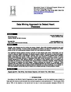
The algorithms and methodologies in this paper were implemented using data from a manufacturer of nurse call devices. The company has four major product families, each comprising hundreds of variant BOMs. For this case study, we used a sample of 405 BOMs from one of the major product families. An example of the part generalization methodology applied to this dataset was shown in Section 3.2; because of space considerations no further discussion of that step will be given here. The subtree generalization algorithm was applied to the single level subtrees in the BOM collection. These 156 single level trees were clustered using CLARANS (Ng and Han, 1994) into subtree clusters, and the individual subassembly part numbers in each BOM replaced with the general labels from this clustering step. The 405 BOMs, clustered using the approach in (Romanowski and Nagi, 2003), were then unified using the GBOM unification algorithm. The unification of one GBOM cluster, using the methodology discussed in Section 3.3, is shown graphically in Figure 12 in UML format. Note the multiplicity ranges for the raw cable (shaded), from 21 to 366 inches, and resin, from 0.01 to 0.05 lbs. Also, this cluster shows a level jump for the plug component (shaded); in 10 out of 25 BOMs the plug is a child of the cable assembly. In BOM #2 the plug is a child of the end item.
20
Cluster 4 N=25 1 1
1 1 ES = .08
ES = 1
CaseFront Assy
1 1 ES = 1
Socket
1 21…366
CaseFront SubAssy
1 1 ES = 1
Case Front
1 2 ES = 1
Fastener
1 1 ES = 1
1 ES =0.4 1 ES(2)=.04
Labor
1 1 ES = 1
Button, Oval
ES = 1
Cable Assy
1 1 ES = 1
ES = 1
Raw Cable
Button, Bar
1 1
Plug
1 1
ES = 1
Box
1 1 ES=.48
Wafer
1 4
ES = 1
Phillips Screw
1 .01…0.05 ES=.84
Resin
1 1 ES = 1
Literature
1 1
Switch
ES = 1
1 1
Speaker/Vol SubAssy
ES = 1
Label
1 1 ES = 1
Vol Assy
1 1 ES = 1
1 1 ES = 1
Bracket
Box Label
1 1 ES = 1
CaseBack SubAssy
Case Back
1 1 ES=.04
Speaker/Vol Assy
1 1 ES = 1
Pin
1 1 ES = 1
1 1 ES = 1
ES = 1
CaseBack Assy
1 6..12 ES=.48
Bracket Assy
1 1 ES = 1
1 1
Knob
1 1
ES = 1
Speaker
1 1 ES = 1
Vol Control
Figure 12: GBOM formed from 25 similar BOMs
3.6 Modeling configuration and design constraints
The last step of modeling the GBOM is determining design rules and configuration constraints. Some rules are common to all BOMs; for instance, the constraint that purchased parts may not have child components, and a child component may not contain its own ancestor. Other rules may be global (common to all products in the domain) or local (common to specific products, and therefore to particular GBOMs). These rules also help define the identifying characteristics of the GBOM cluster. The process of forming the GBOM generates topological, configuration, and multiplicity constraints, as seen in the UML diagram in Figure 12. Other rules, such as those involving specific part characteristics, must be derived using other methods. Association mining algorithms (Agrawal et al., 1993; Zaki, 2000; Liu et al., 1998) that look for frequently occurring itemsets in a database are an appropriate tool for this task. A typical design association rule might be “If the car type is compact, the engine type is 4 cylinder.” The strength of association in these itemsets is quantified by two measuress: support (the percentage of records containing the antecedent) and confidence (the percentage of records containing the antecedent that also contain the consequent). The values of these measures, which are set by the user, directly affect the number of rules generated by the algorithm. Finding global rules requires mining over all BOMs in the product database; we do not address that issue in this paper. To find local rules, each cluster of BOMs is mined separately. 21
For this task, the part descriptions are necessary as they provide information on the critical characteristics of each component. Association mining data are in the form of a comma-separated set of records; for this BOM application, these data are similar to a parts list but use short descriptors instead of unique ID numbers. For instance, Figure 13 shows a record for one of the 25 BOMs contained in the GBOM in Figure 11. The parts are identified using short string versions of the part descriptions (e.g., BarButton, OvalButton) based on the generalization results from Section 3.4.2. Note that in this domain, the number of parts in a BOM is fairly small; however, if the number of parts is much larger than the number of records, some method of factor reduction must be used. CaseFAssy,BrackAssy1sw,ZincBrack,PushMomSw,CFGen2,BarButton,OvalButton,SpkVCAssy205808, VolContAssy,200VC,Gen2Knob,8OSpkr,10ftCableAssy,R3Cond22,PVCResin,602Pin6,5PinWafer,Labor,Poly, CaseBAssy,CBGen2,Label,Box,Phillips1in,2InChain,Lit
Figure 13: Example association mining record
The output of a mining algorithm may include interesting, novel patterns but also trivial and already known relationships. Domain knowledge and user input is required to sift through and validate the rules included in the constraints. One major benefit of a data mining approach is the reduced need for user engagement, which is focused primarily on the verification and validation of induced rules instead of their generation. This methodology promotes automation of activities and tasks that do not require human intervention, and thus frees this expensive and constrained resource for the tasks where human expertise and effort are most important. For Cluster 4, with a minimum support of 30%, and minimum confidence of 50%, 2025 rules were generated – many of which were, as expected, trivial or redundant. The rules characterize this cluster as a two-button G2 pillow speaker (TV and nurse), with a 200 Ohm volume control. The major variations from this base model are the length of the cable (48% have an 8 ft cable) and the speaker (60% have a 3.2 Ohm speaker and the remaining 40% use an 8 Ohm speaker). A sample rule generated by CBA (Classification Based on Association), an association and classification program developed by (Liu, Hsu and Ma, 1998) based on the Apriori algorithm (Agrawal et al., 1993) is shown in Figure 14. The rule is read as “IF 8 ft cable assembly is present, THEN 3.2 Ohm speaker is also present.” The numerical results following the rule represent the support, confidence, number of records containing the attribute “8ftCableAssy”, number of attributes containing “32OSpkr”, and the ratio of support to confidence. The support is calculated by dividing the number of records containing the
22
precedent (12) by the total number of records in the dataset (25), which is 48%. The confidence is the number of records containing both the precedent and the antecedent (8) divided by the number of records containing the precedent (12), which equals 66.67%. In contrast, mining the 6 BOMs in Cluster 8 (whose GBOM is shown below in Figure 15) generates rules showing this family of products can be characterized as a four-button pillow speaker with an 8 foot, 24 gauge cable; the major variations are in the printing for the buttons and in the volume control (75 to 10000 Ohm) and speaker (8 and 40 Ohm) components. Rule 8: 8ftCableAssy = Y -> 32OSpkr = Y (48.000% 66.67% 12 8 32.000%)
Figure 14: Example association mining rule
Cluster 8 N=6
1 1 ES =0.17 Resistor
1 1 ES = 1
1 1 ES = 1 CaseFront Assy
Fastener
1 1 ES = 1
1 1 ES = 1 Case Front
1 4 ES=1 Switch
1 1 ES = 1 Bracket Assy
1 1 ES = 1
1 2 ES=1 Bracket
1 1 ES = 1
1 1 ES = 1 Pin
Button Oval
1 4 ES = 1 Spring
Plastite Screw
Raw Cable
CaseFront SubAssy
1 1 ES = 1
1 4 ES = 1
1 1 ES = 1 Labor
1 1 1 ES=0.83 1 ES=1 Button Sq, Grey
Speaker
Pad
1 1 ES = 1
1 1 ES = 1
Cable Assy
Literature
1 1 1 1 1 ES=0.5 1 ES=1 0.1..0.11 ES=1 1..12 ES = 1 Plug
1 4 ES = 1 Spring
Wafer
1 1 ES = 1 Screw
Resin
Pin
1 1 1 ES=0.17 2 ES = 1 Button Printed
1 1 ES = 1 Button Square
Button Printed
1 1 ES = 1
1 1 ES = 1
Box
CaseBack Assy
1 1 ES=0.33 Protector
1 1 ES = 1
1 1 ES = 1 CaseBack SubAssy
1 1 ES = 1 Case Back
Vol Control Assy
1 1 1 ES = 1 1 ES=1 Knob
Labor
1 1 ES=1 Vol Control
1 1 ES = 1 Label
1 1 ES = 1 Button End
Figure 15: A GBOM formed from 6 similar BOMs
3.6 CXML representation of GBOMs and constraints
The intent of GBOM representations is to maintain structural information and avoid redundancy while incorporating design information into a compact form. We can exploit these characteristics of GBOMs in the search for similar parts, taking advantage of the reduced search space resulting from the decrease in redundant information. We also, by representing GBOMs as
23
constrained XML files, take advantage of the characteristics of XML as a framework for data storage. Constrained XML extends the XML language to include restrictions of many types on the XML file contents. For example, constraints common to all bills of material include: •
restrictions on the quantity per field (for instance, there can be only one end item)
•
restrictions on the number of children (purchased parts may not, by definition, have children)
•
restrictions on node relationships (for instance, a node may not be a child of itself)
•
checks on correctness (for instance, the cost of a parent item should equal the cost of its children multiplied by their respective quantities, plus added labor costs of assembling/processing the parent).
•
checks on validity of part numbers.
Specific constraints may also be written for a particular domain to maintain completeness, consistency, and correctness of BOM files. For instance, we can include •
restrictions on which parts can be substituted
•
restrictions on vendor choice
•
restrictions on configuration (for example, which parts can be used together in an assembly, and which are incompatible)
•
validation of BOM contents (for example, ensuring that all necessary part types are included and the BOM is complete).
These constraints are included in the document type definition (DTD) file (see McKernon and Jayaraman, 2000, for a discussion on the advantages of using DTDs over XML Schema). Individual XML files written to the specifications in the DTD are parsed first for compliance with XML formats, and second for compliance with the constraints. In this manner, we can enforce consistency, correctness, and completeness of BOMs, which can further enhance search effectiveness and efficiency. While the GBOMs could be shown as graphs instead of trees by explicitly adding the alternate edges resulting from differing ancestry relationships, we have chosen to use the XML representation for its portability across disparate platforms. XML documents are also tree structures, which nicely supports the conversion of GBOM information into an XML file. The DTD file, made up of elements and attributes (and, in the CXML extension, constraints) spells out the relationships between the parts of the document tree. Elements represent nodes in the
24
tree; each DTD has one and only one root element (see Figure 16, where the root element is ‘PillowSpeaker’). Elements may include other elements, and occurrence operators such as * and + designate how many of each child element can appear in the document. If no operator is present, the element appears once and only once. An asterisk means an element can appear zero or more times. A + symbol means the element must appear at least once, but can appear more than once. #PCDATA stands for parsed character data. Attributes are either required or implied; implied attributes do not need to appear in the XML document. In this example, the attributes are all character data (CDATA) although enumerated types and tokenized types are also allowed. Figure 16 contains four constraints: the first constraint lists an alternate parent for a particular item number. The second constraint checks the quantity per parent; the third constraint makes sure all variants are included in the XML file, and the fourth constraint checks for completeness. A more extensive encoding of assembly compatibility and design configuration constraints within the CXML framework is proposed as a research agenda in (Romanowski and Nagi, 2001). See the appendix for further discussion of DTD formulations, a CXML version of the GBOM in Figure 12, and an example CXML parser output.
(Item_no+, Box, CableAssy, CaseBackAssy, CaseFrontAssy, Hardware, Lit, Plug, Socket, SpeakerVolAssy)>
#REQUIRED> (IDnum,Cardinality,Alt_Parent)> #REQUIRED> (#PCDATA)> (#PCDATA)> (#PCDATA)> (Item_no+)> (Item_no+, Labor, Pin*, Plug*, RawCable, Resin*, Wafer*)> (Item_no+, CBSubAssy)> (Item_no+, CFSubAssy)> (Item_no+, SpeakerVolSubAssy)> (Item_no+, Button, BracketAssy, CaseFront)> (Item_no+, CaseBack, Label)> (Item_no+, Speaker, VolAssy)> (Item_no+, Hardware, Labor*, Switch)> (Item_no+, Knob, VolControl)> (Item_no+)> (Item_no+)> (Item_no+)>
IF EXISTS (PillowSpeaker.CableAssy.Plug.item_no == PL-060) /* Designates alternate parent for plug item PillowSpeaker.CableAssy.Plug.item_no.Alt_Parent = 103-011> IF EXISTS (PillowSpeaker.CableAssy.Resin.item_no == PolyR110) /* Checks for correct quantity per parent PillowSpeaker.CableAssy.Resin.item_no.Cardinality = 0.011> SUM(PillowSpeaker.CableAssy.RawCable:strength)==1> /* Checks for inclusion of all variant items SETOF(PillowSpeaker.CableAssy.Resin)=S AND size(S)==2> /* Checks for completeness, must have two items from the Resin group
]
Figure 16: Sample GBOM DTD with constraints 25
4. Summary and future work
This paper presented a novel data mining-based methodology for semi-automated formation of a generic bill of materials from legacy BOMs. The methodology is a systematic approach for the problems of unifying similar, but not identical, trees into a single entity. In summary, we develop a method for generalizing parts and subassemblies using text mining; present an algorithm for unifying similar BOM tree structures into a single GBOM; and extract design and configuration rules from the BOM data using association mining. These data mining-based methodologies for generalizing parts and subassemblies and unifying similar BOMs are illustrated using data from an industrial BOM database. The resulting GBOMs, which contain information on the most common product structure and variations of that structure, reduce the search space for retrieving similar previous designs and aid in configuring new variants. We represent the GBOMs in platform independent, constrained XML to support distributed and virtual enterprises. Some future directions for data mining-based research in this area include: •
developing a hybrid text/numerical mining algorithm to efficiently mine part description fields, which typically contain many different data types. For example, the description “SPACER,ENHANCED,1/4",HI-IMPACT POLYSTYRN” contains categorical (SPACER, HI-IMPACT POLYSTRN), numerical (1/4”),and ordinal (ENHANCED) data types. No algorithm currently exists to mine all possible data types simultaneously. Such an algorithm can also be applied to other manufacturing documents such as process plans and routings; the knowledge mined from these information sources can then be integrated into the GBOM.
•
refining of the distance measure to increase efficiency of the tree clustering process. The current measure can overstate distances for some configurations where identical child items have different parents (see Romanowski, Nagi and Sudit, 2003).
•
deriving design and configuration constraints from mining of related product documents such as CAD drawings, R&D reports, production records, etc., and representing those constraints in CXML. Data mining offers many attractive solution methods for difficult information-related
engineering problems. As shown in this paper, these methods can greatly reduce the amount of human effort required for tedious tasks, freeing up resources for more critical functions such as validation and verification, that are best performed by domain experts.
26
References Agrawal, R., T. Imielinski, A. Swami, 1993, “Mining association rules between sets of items in large databases,” SIGMOD Record (ACM Special Interest Group on Management of Data), 22(2): 207-216.
Cook, D. J. and L. B. Holder, 2000, “Graph-Based Data Mining,” IEEE Intelligent Systems, 15(2): 32-41. Farrell, R. and T. Simpson, 2003, “Product platform design to improve commonality in custom products,” Journal of Intelligent Manufacturing, 14 (6): 541-556. Ham, I., K. Hitomi, and T. Yoshida, 1985, Group Technology: Applications to Production Management (International Series in Management Science/Operations Research, 9), Kluwer Academic Publishers. Ham, I., D. Marion, and J. Rubinovich, 1986, “Developing a Group Technology Coding and Classification Scheme,” Industrial Engineering, 18(7): 90-97. Harhalakis, G., A. Kinsey, and I. Minis, 1992, “Automated Group Technology Code Generation Using PDES,” in Proc. 3rd Int. Conf. Computer Integrated Manufacturing, Rensselaer Polytechnic Institute, Troy NY. Hegge, H. M. H., and Wortmann, J.C., 1991, “Generic bill-of-material: a new product model,” International Journal of Production Economics, 23: 117-128. Henderson, M. and S. Musti, 1988, “Automated Group Technology Part Coding from a ThreeDimensional CAD Database,” Journal of Engineering for Industry, 110(3): 278-287. Iyer, S. and R. Nagi, 1997, "Automated Retrieval and Ranking of Similar Parts in Agile Manufacturing," IIE Transactions, Design and Manufacturing, special issue on Agile Manufacturing, 29(10): 859-876. Jiao, J. and M.M. Tseng, 1999a, “Methodology of developing product family architecture for mass customization,” Journal of Intelligent Manufacturing, 10(1): 3-20 Jiao, J., M.M. Tseng, Q. Ma, and Y. Zou, 2000, “Generic Bill-of-Materials-and-Operations for high-variety production management,” Concurrent Engineering-Research & Applications, 8(4): 297-321. Kao, Y., and Y.B. Moon, 1991, “Unified Group Technology implementation using the backpropagation learning rule of neural networks,” Computers & Industrial Engineering, 20(4): 425-437. Koenig, D. T., 1994, Manufacturing engineering: principles for optimization, Washington, D.C.: Taylor & Francis. Lee-Post, A., 2000, “Part family identification using a simple genetic algorithm,” International Journal of Production Research. 38(4): 793-810. Liu, B., W. Hsu, Y. Ma, 1998, "Integrating Classification and Association Rule Mining." Proceedings of the Fourth International Conference on Knowledge Discovery and Data Mining (KDD-98, Plenary Presentation), New York, USA.
27
McKernan, T. J. and B. Jayaraman, 2000, “CobWeb: A Constraint-based XML for the Web”, Department of Computer Science, University at Buffalo. Ng, R. and J. Han, 1994, "Efficient and Effective Clustering Methods for Spatial Data Mining", Proceedings of 20th International Conference on Very Large DataBases, pp 144-155. Opitz, H., 1970, A Classification System to Describe Workpieces (translated by A. Taylor), New York: Pergamon Press. Orlicky, J., 1995, Material Requirements Planning, New York: McGraw-Hill Book Company. Prebil, I., S. Zupan, P. Lu, 1995, “Adaptive and Variant Design of Rotational Connections,” Engineering with Computers 11: 83-93. Ramabhatta, V., L. Lin and R. Nagi, 1997, “Object Hierarchies to aid Representation and Variant Design of Complex Assemblies in an Agile Environment,” International Journal of Agile Manufacturing 1(1): 77-90. Romanowski, C.J. and R. Nagi, 2003, “On comparing bills of materials: A similarity/distance measure for unordered trees,” accepted by IEEE Transactions on Systems, Man, and Cybernetics, Part A. Romanowski, C.J. and R. Nagi, 2001, “A Data Mining-Based Engineering Design Support System: A Research Agenda,” in Data Mining for Design and Manufacturing: Methods and Applications, D. Braha, ed., Kluwer Academic Publishers, pp. 235-254. Romanowski, C.J. and R. Nagi, 2004, “Adaptive data mining in a variant design support system”, in Proceedings of the 13th Industrial Engineering Research Conference, Houston TX. Romanowski, C.J., R. Nagi, and M. Sudit, 2003, “Data mining in an engineering design environment: OR applications from graph matching,” submitted to Computers and Operations Research, special issue on Data Mining. Shah, J. and A. Bhatnagar, 1989, “Group Technology Classification from Feature-Based Geometric Models,” Manufacturing Review, 2(3): 204-213. Simpson, T., K. Umapathy, J. Nanda, S. Halbe, B. Hodge, 2003,“Development of a Framework for Web-based Product Platform Customization,” Journal of Computing and Information Science in Engineering, 3:119-129. Zaki, Mohammed J., 2000, “Scalable algorithms for association mining,” IEEE Transactions on Knowledge & Data Engineering, 12(3): 372-390.
28
Appendix A. The search for similar parts
To place this research into context, this section discusses how the CXML representation of the GBOM can be searched for similar parts and subassemblies. Table 1a shows the typical search types, their parameters, and expected outputs. Table 1a: Typical searches for design re-use
Search Type Where used Similar parts Similar subassemblies/ components Similar product
Search for
Parameters
Output
Specific item Items Items
Item Number Item description Content and topology
List of ancestor items List of items with BOM links Subtrees with BOM links
End item
End item description, content, topology
Bills of material; a recursive version of the subassembly search
The search for similar subassemblies begins with the definition of desired attribute values. The values are compared with previously defined group characteristics, and the most similar groups – subject to a user-defined threshold for similarity – are identified as ranked candidate groups. The XQuery search is run, using these ranked candidate groups, and the results displayed for the user. Figure 1a shows the search process. B. Maintaining design feasibility
When using the results from a search to configure a new
Search for similar subassembly
variant, the lower level parts and subassemblies chosen should maintain the design’s feasibility. The GBOMs are determined from existing, established product designs. The GBOM
Define desired attribute values Group characteristics and similarity values
generation process captures configuration constraints, such as cardinality and parent-child relationships, that are subsequently included in the GBOM DTD file. Additionally, association mining of the individual BOMs contributes more constraints in
Determine candidate groups
Run query, searching for candidate groups
the form of specific component attributes. The combination of general and specific constraints provides a DTD that completely specifies the product design. As a check on feasibility, an XML
Rank and display results
Figure 1a: Search procedure
file of the new product variant can be sent to the constrained XML parser; violations of domain-specific constraints will be flagged in the process. Therefore, 29
the CXML parser would recognize a bicycle BOM missing the rear brake assembly. Design rule constraints check for feasible combinations; the CXML parser would recognize that a 4-cylinder engine requires 4 pistons of a specific bore and compression ratio. C. DTDs and CXML files for GBOMs
The GBOM, because it is a union of several BOMs, requires a DTD that is a modification of an individual BOM DTD. In this DTD, we are concerned with being able to search for similar parts, purchased parts, and subassemblies; we also want to make sure the combinations of components and subassemblies form a valid end product. Also, clustering – both by content and by topology – forms groups of similar items, so we use these group definitions to support the similar component search. Completeness and correctness are checked using XML occurrence operators and design rules are represented as constraints. Figure 2a shows a portion of a CXML file for the GBOM in Figure 11 (section 3.4), corresponding to the DTD in Figure 16. Figure 3a shows the output from the CXML parser.
1038 1 BX10 1 8ftCableAssy 1 Str020 1 PVC100 0.01 PolyR110 0.011
Figure 2a: CXML file for GBOM in Figure 11
30
> java CxmlUI clus4.xml There were no XML Syntax Errors. There were no CXML Semantic Constraint Violations. Executed CXML Instructions: 0: 2.0 eq 1: 1.0 eq 2: 2.0 eq 3: 1.0 eq 4: 1.0 eq 5: 4.0 eq 6: EXISTS
2.0 1 -2 1.0 2 -2 2.0 3 -2 1.0 4 -2 1.0 5 -2 4.0 6 -2 PillowSpeaker.CableAssy.Plug.item_no.IDnum eq PL60 7 -2
Figure 3a: CXML parser results for CXML file
31