Detection of Online Financial Transaction. Dr. Jyotindra N. Dharwa. Dr. Ashok R. Patel. Asst. Professor,. Director,. A. M. Patel Institute of Computer Studies,.
International Journal of Computer Applications (0975 – 8887) Volume 16– No.1, February 2011
A Data Mining with Hybrid Approach Based Transaction Risk Score Generation Model (TRSGM) for Fraud Detection of Online Financial Transaction Dr. Jyotindra N. Dharwa Asst. Professor, A. M. Patel Institute of Computer Studies, Ganpat University, Kherva, India.
ABSTRACT We propose a unique and hybrid approach containing data mining techniques, artificial intelligence and statistics in a single platform for fraud detection of online financial transaction, which combines evidences from current as well as past behavior. The proposed transaction risk generation model (TRSGM) consists of five major components, namely, DBSCAN algorithm, Linear equation, Rules, Data Warehouse and Bayes theorem. DBSCAN algorithm is used to form the clusters of past transaction amounts of the customer, find out the deviation of new incoming transaction amount and finds cluster coverage. The patterns generated by Transaction Pattern Generation Tool (TPGT) are used in Linear equation along with its weightage to generate a risk score for new incoming transaction. The guidelines shown in various web sites, print and electronic media as indication of online fraudulent transaction for Credit Card Company is implemented as rules in TRSGM. In the first four components, we determine the suspicion level of each incoming transaction based on the extent of its deviation from good pattern. The transaction is classified as genuine, fraudulent or suspicious depending on this initial belief. Once a transaction is found to be suspicious, belief is further strengthened or weakened according to its similarity with fraudulent or normal transaction history using Bayes theorem.
Keywords Data Mining, FDS, Cyber Crime, Credit Card, Bayes Theorem
1. INTRODUCTION The Internet all over the world is growing rapidly. It has given rise to new opportunities in every field we can think of - be it entertainment, business, sports or education. There are two sides to a coin. Internet also has its own disadvantages. One of the major disadvantages is Cyber crime- illegal activity committed on the internet. The internet, along with its disadvantages, has also exposed us to security risks that come with connecting to a large network. Computers today are being misused for illegal activities like e-mail espionage, credit card fraud, spasm, software piracy and so on, which invade our privacy and offend our senses. Criminal activities in the cyberspace are on the rise. According to Internet Crime Report of Internet Crime Complaint Center, there was a 33.1% increase of cyber crime cases in 2008 as compared to 2007 [1]. A key area of interest regarding Internet fraud is the average monetary loss incurred by complainants contacting IC3. Of the 72,940 fraudulent referrals processed by IC3 during 2008, 63,382 involved a victim who reported a monetary loss. The total dollar loss from all referred cases of
Dr. Ashok R. Patel Director, Department of Computer Science Hem. North Gujarat University, Patan, India
fraud in 2008 was $264.6 million. A Gartner survey of more than 160 companies reveals that 12 times more fraud exists on Internet transactions than other offline transactions [2].According to the Cybersource, 11th Annual Online Fraud Report, which is based on U.S.A. and Canadian online merchants, from 2006 to 2008 the percent of online revenues lost to payment fraud was stable [3]. However, total dollar losses from online payment fraud in the U.S. and Canada steadily increased during this period as ecommerce continued to grow. To address this problem, financial institutions use various fraud prevention tools like real-time credit card authorization, address verification systems (AVS), card verification codes, rule-based detection, etc. But fraudsters are intelligent and devise new ways to escape from such protection mechanisms. The main concern is that such kind of money can be used in other criminal or terrorist activities. Thus once fraud prevention failed, and then there is a need of effective system to detect fraud. Developing a financial cyber crime detection system is a challenging task. Whenever any online transaction is performed through the credit card, then there is no any system that surely predicts any transaction as fraudulent. It just predicts the likelihood of the transaction to be a fraudulent.
2. RELATED WORK There are various approaches used in credit card fraud detection namely neural network, data mining, meta-learning, game theory and support vector machine. Gosh and Reilly [4] have developed fraud detection system with neural network. Their system is trained on large sample of labeled credit card account transactions. These transactions contain example fraud cases due to lost cards, stolen cards, application fraud, counterfeit fraud, mail-order fraud and non receive issue(NRI) fraud. Aleskerov et al. [5] present CARDWATCH, a database mining system used for credit card fraud detection. The system is based on a neural learning module and provides an interface to variety of commercial databases .Dorronsoro et al. [6] have suggested two particular characteristics regarding fraud detection- a very limited time span for decisions and a large number of credit card operations to be processed. They have separated fraudulent operations from the normal ones by using Fisher’s discriminant analysis. Syeda et al. [7] have used parallel granular neural network for improving the speed of data mining and knowledge discovery in credit card fraud detection. A complete system has been implemented for this purpose. Chan et al. [8] have divided a large set of transactions into smaller subsets and then apply distributed
18
International Journal of Computer Applications (0975 – 8887) Volume 16– No.1, February 2011 data mining for building models of user behavior. The resultant base models are then combined to generate a meta-classifier for improving detection accuracy. V.Hanagandi et al. [9] generate a fraud score using the historical information on credit card account transactions. They describe a fraud-non fraud classification methodology using radial basis function network (RBFN) with a density based clustering approach. The input data is transformed into cardinal component space and clustering as well as RBFN modeling is done using a few cardinal components. A.Shen et al. [10] investigates the efficacy of applying classification models to credit card fraud detection problems. They tested three classification methods i.e. neural network, decision tree and logistic regression for their applicability in fraud detections. H.shao et al. [11] introduced an application in data mining to detect fraud behavior in customs declarations data and used data mining technology such as an easy-to-expand multi-dimensioncriterion data model and a hybrid fraud-detection strategy. A. Srivastava et al. [12] model the sequence of operations in credit card transaction processing using Hidden Markov Model (HMM) and show how it can be used for detection of frauds. An HMM is initially trained with normal behavior of card holder. If an incoming credit card transaction is not accepted by trained HMM with sufficiently high probability, it is considered to be fraudulent. At the same time they also try to ensure that genuine transactions are not rejected. J.Quah et al. [13] focuses on real time fraud detection and presents a new and innovative approach in understanding spending patterns to decipher potential fraud cases. They make use of self organizing map to decipher, filter and analyze customer behavior for detection of fraud. Recently fraud detection system is developed by Suvasini Panigrahi et al. [14], which consist of four components, namely, rule-based filter, Dempster-Shafer adder, transaction history database and Bayesian rule. In the rule based component, they determine the suspicion level of each incoming transaction based on the extent of its deviation from good pattern. Dempster-Shafer theory is used to combine multiple such evidences and an initial belief is computed. S.J.Stoflo et al. [15] developed the JAM distributed data mining system for the real world problem of fraud detection in financial information systems. They have shown that cost-based metrics are more relevant in certain domains, and defining such metrics poses significant and interesting research questions both in evaluating systems and alternative models, and in formalizing the problems to which one may wish to apply data mining technologies. Researchers also published some survey papers in the area of fraud detection. Phua et al. [16] presented a comprehensive report using an extensive survey of data mining based Fraud Detection Systems and. Kou et al. [17] have compared and measured performance of various fraud detection techniques for credit card fraud, telecommunication fraud and computer intrusion detection. Bolton and Hand [18] identified the tools available for statistical fraud detection and areas in which fraud detection technologies are most commonly used. D.W.Abbott et al. [19] compare five of the most highly acclaimed commercial data mining tools on a fraud detection application, with descriptions of their distinctive strengths and weaknesses, based on the lessons learned by the authors during the process of evaluating the products. There are two types of data mining techniques, Unsupervised and Supervised Methods. Unsupervised methods do not need the prior knowledge of fraudulent and non-fraudulent transactions in historical database, but instead detect changes in behavior or unusual transactions. Supervised methods require accurate
identification of fraudulent transactions in historical databases and can only be used to detect frauds of a type that have previously occurred. An advantage of using unsupervised methods over supervised methods is that previously undiscovered types of fraud may be detected. The main concern in this domain is that genuine transaction might not be caught as fraudulent transaction otherwise it creates inconvenience and dissatisfaction to customer. In the same way, fraudulent transaction should not go undetected otherwise the financial company has to suffer lot of money. It is well known that every card holder has certain purchasing habits. Generally they repeat their shopping habits. Most of the FDS try to find the deviation from this good pattern by only implementing rules or with the similarity from past fraudulent transaction set. However these rules are largely static in nature, if fraudsters develop or learn new methods and tactics to evade detection by FDS, then new types of fraud may get unnoticed. Thus system which is not dynamic and able is adapt to new change, may become outdated resulting in large number of false alarms. So there is a need of developing new system which integrates all the multiple evidences of past genuine and fraudulent transaction set and also focus current dynamic behavior of customer. We propose a hybrid model containing data mining techniques, statistics and artificial intelligence to collect and combine all the multiple evidences. The model not only considers the past behavior but also monitors the current behavior very closely. The current behavior is stored in the different lookup tables. Whenever any deviation other than normal behavior found it is further checked with fraudulent transaction history with bayes theorem. To the best of our knowledge, this is first ever attempt to develop financial cyber crime detection system using hybrid approach like data mining, statistics and artificial intelligence. The rest of paper is organized as follows. We discuss the transaction pattern generation tool in brief in section 3. Section 4 describes proposed transaction risk score generation model along with its methodology. Section 5 shows the result as scatter graph in terms of clusters formed by DBSCAN algorithm. Implementation environment and result analysis & discussions are covered in section 6 and 7 respectively. Finally we conclude in section 8.
3. TRANSACTION PATTERN GENERATION TOOL The transaction pattern generation tool (TPGT) will generate the patterns (parameters) based on the historical data stored in the data warehouse. TPGT is implemented in the Oracle 9i. All the patterns generated by TPGT will collectively decide the purchasing behavior of the card holder. These patterns are very useful for deciding or verifying the current transaction performed by the card holder online. It generates more than 60 parameters. As this domain is sensitive and due to space limitation, it is not possible to discuss each parameter. Here are the main parameters generated by TPGT.
3.1 Main Patterns (Parameters) Generated by TPGT DP: Daily Parameters, CP: Category Parameters, PP: Product Parameters, TP: Transaction Parameters, WP: Weekly Parameters, VP: Vendor Parameters, AP: Address Parameters, FP: Fortnightly Parameters, MP: Monthly Parameters, SP: Sunday Parameters,
19
International Journal of Computer Applications (0975 – 8887) Volume 16– No.1, February 2011 HP: Holiday Parameters, LP: Location Parameters, GP: Transaction Gap Parameters
3.2 Computations of the Patterns 3.2.1 TP1 to TP8 The Calculation of the parameters TP1 to TP8 in the tool is done as follows. The tool divides all the transactions of the customer into eight different time frames according to the following. T1 becomes true if the past transaction is performed from 3:00 to 6:00 time frame on the card Ck within data warehouse. T 1 TRUE | { Tck 3 : 00 t 6 : 00} (1) T2 becomes true if the past transaction is performed from 6:00 to 9:00 time frame on the card Ck within data warehouse. T 2 TRUE | { Tck 6 : 00 t 9 : 00} (2) T3 becomes true if the past transaction is performed from 9:00 to 12:00 time frame on the card Ck within data warehouse. T 3 TRUE | { Tck 9 : 00 t 12 : 00} (3) T4 becomes true if the past transaction is performed from 12:00 to 15:00 time frame on the card Ck within data warehouse. (4) T 4 TRUE | { Tck 12 : 00 t 15 : 00} T5 becomes true if the past transaction is performed from 15:00 to 18:00 time frame on the card Ck within data warehouse. (5) T 5 TRUE | { Tck 15 : 00 t 18 : 00} T6 becomes true if the past transaction is performed from 18:00 to 21:00 time frame on the card Ck within data warehouse. (6) T 6 TRUE | { Tck 18 : 00 t 21: 00} T7 becomes true if the past transaction is performed from 21:00 to 0:00 time frames on the card Ck within data warehouse. T 7 TRUE | { Tck 21: 00 t 0 : 00} (7) T8 becomes true if the past transaction is performed from 0:00 to 3:00 time frame on the card Ck within data warehouse.
T 8 TRUE | { Tck 0 : 00 t 3 : 00}
(8) The tool then finds the total number of the transactions performed by the customer in time frame from T1 to T8. TPi = occurrences (count) of Ti on the card Ck from the data warehouse, where 1 i 8 (9) Finally the percentage of all the parameters of all the transactions is computed as follows. Percent_TPi=(TPi * 100) / total transactions on card Ck from the data warehouse, where 1 i 8 (10) Convert_time () function is also implemented to map time of one city to another city with time zone. So customer performs overseas transaction then also time is converted accordingly.
3.2.2 TP11 and TP12 L1 becomes true if the transaction is performed from 0:00 to 4:00 on the card Ck from the data warehouse. L1 TRUE | { Tck 0 : 00 t 4 : 00} (11) L2 becomes true if the transaction is performed except from 0:00 to 4:00 on the card Ck within the data warehouse. L2 TRUE | { Tck 4 : 00 t 0 : 00} (12) Finally TP11 and TP12 are computed as follows. TP1i = occurrences (count) of Li on the card Ck from the data warehouse where 1 i 2 (13)
3.2.3 GP1 to GP7 G1 becomes true if the transaction occurs just within 4 hours from the previous transaction on the same card Ck from the data warehouse. (14) G1 True | {Tck (0 d 4)} d stands for the duration in hours between two successive transactions. G2 becomes true if the transaction occurs just within 5 to 8 hours from the previous transaction on the same card C k from the data warehouse. (15) G 2 True | {Tck (4 d 8)} G3 becomes true if the transaction occurs just within 9 to 16 hours from the previous transaction on the same card Ck from the data warehouse. (16) G3 True | {Tck (8 d 16)} G4 becomes true if the transaction occurs just within 17 to 24 hours from the previous transaction on the same card C k from the data warehouse. (17) G 4 True | {Tck (16 d 24)} G5 becomes true if the transaction occurs from 2 nd day to within a week from the previous transaction on the same card Ck from the data warehouse. (18) G5 True | {Tck (24 d (24 * 7))} G6 becomes true if the transaction occurs just within 15 days from the second week since the previous transaction on the same card Ck from the data warehouse. (19) G 6 True | {Tck ((24 * 7) d (24 *15))} G7 becomes true if the transaction occurs after 15 days from the previous transaction on the same card Ck from the data warehouse. (20) G 7 True | {Tck (d (24 *15))} Now the parameters GP1 to GP7 are computed as follows. GPi = occurrences (count) of Gi on the card Ck from the data warehouse, where 1 i 7 (21) (8)
3.2.4 AP1 and AP2
A1 becomes true if the past transactions are also shipped with the same shipping address from the data warehouse. (22) A1 TRUE | { Tck Saddr (Tcurrent ) Saddr ( Tpast ) } A2 becomes true if the transaction is performed with the different shipping and billing address. (23) A2 TRUE | { Tck Saddr Baddr } Finally AP1 and AP2 are computed as follows. APi = occurrences (count) of Ai on the card Ck from the data warehouse, where 1 i 2 (24) Other parameters are computed in the similar way.
4. PROPOSED TRANSACTION RISK SCORE GENERATION MODEL (TRSGM) In the TRSGM, a number of rules are used to analyze the deviation of each incoming transaction from the normal profile of the cardholder by computing the patterns generated by TPGT. The initial belief value is obtained as the risk score. The model also considers the transaction whether it is performed on normal working day, Sunday or holiday. It will match the past transaction behavior on the similar type of day and accordingly it generates a risk score. The initial belief is further strengthened or weakened according to its similarity with fraudulent or genuine transaction history using Bayes theorem. In order to meet this functionality,
20
International Journal of Computer Applications (0975 – 8887) Volume 16– No.1, February 2011 the TRSGM is designed with the following five major components: (1) DBSCAN algorithm, (2) Linear equation, (3) Rules, (4) Data Warehouse and (5) Bayes theorem
4.1 DBSCAN algorithm A customer usually carries out similar types of transactions in terms of amount, which can be visualized as part of a cluster. Since a fraudster is likely to deviate from the customer’s profile, his transactions can be detected as exceptions to the cluster – a process known as outlier detection. It has important applications in the field of fraud detection and has been used for quite some time to detect anomalous behavior. Here DBSCAN algorithm is used to form the clusters of transaction amounts spend by the customer. Whenever a new transaction is performed by the customer, the algorithm finds the cluster coverage of this particular amount. If this amount occurs more than once in the past, then the TRSGM considers as highly genuine transaction. Result of Implementation of DBSCAN algorithm as scatter graph is shown in Fig.1.
4.2 Linear Equation The TRSGM is based on the following linear equation, which generates a risk score and indicates how far or close the current transaction is from the normal profile of the customer. If the generated risk score is closer to 0, then it is considered closely match to customer normal profile. If the risk score is greater than 0.5 or close to 1, then it considered heavily deviation from the customer normal profile. n
Risk score (1 thresold )
( P *W ) i
i
(25)
i 1
Where threshold=0.5, Pi = Parameter generated by TPGT, Wi= Weightage of the parameter which is given as input to algorithm 1, Weightage is in the percentage
4.2.1 Parameters Sr No 1 2 3 4 5 6 7 8 9 10
Table 1 Parameters of the Equation Parameter Location from which product is ordered Amount of the transaction Number of the transactions Category of the purchase Time frame during which product is ordered Seller or Vendor, with whom product is purchased Same product purchased within short time Time passed since the last transaction Late night transaction Overseas transaction
Weightage W1 % W2 % W3 % W4 % W5 % W6 % W7 % W8 % W9 % W10 %
4.2.2 Formation of Linear Equation The sigmoid function is computed as: f(x)=1/1+e –x (26) where e is the base of natural logarithms approx. by 2.718282. This function is used when the value of parameter can not be shown in the percentage as it maps the computation value in the range [0, 1]. The equation is a linear combination of the following sub equations.
1. ( 1 – percentage_location_count / 100) * W1 (27) 2. ( ( 1 – percentage_category_amount / 100) * W4) / no_of_product_purchased) (28) 3. ( 1 / ( 1 + e –x) ) * W2 (29) where x = (current_transaction_amount – max_transaction_amount) * 25 / current_transaction_amount 4. ( 1 / ( 1 + e –x) ) * W3 (30) where x = (current_transaction_total – max_transaction_total) * 25 / ( 7 * current_transaction_total) 5. (1 – time_percentage / 100) * W5 (31) 6. ((1 – seller_amount_percentage / 100) * W6) / (no_of_product_purchased) (32) 7. (1 / (1 + e –x) ) * W7 (33) where x = (1620 – time_same_product) / ( time_same_product * 0.005 ) 8. (1 / ( 1 + e –x) ) * W8 (34) where x = time_last_transaction / 75 9. (1 – latenight_transaction_percentage / 100) * W9 (35) 10. (1- overseas_transaction_percentage / 100) * W10 (36) The co-efficient of sigmoid function is derived by creating a small simulator programs and exhaustive run of the same. The weightage of different parameters have been derived and implemented using artificial intelligence. Despite that the application is not stick to this weightage, it is made dynamic and can be changed if any credit card company wish to do that. It is also observed that within particular month or time, fraudster becomes so active and fraudulent transactions increased drastically. So it is useful as the weightage is dynamic because we can give more weightage to any sensitive parameter when there is a fear of fraudster in a particular time period. Due to sensitivity of the topic and security reason, actual weightage can’t be disclosed in public.
4.3 Rules There are various guidelines given on several websites, print and electronic media as indications of fraudulent transaction. These guidelines are implemented as rules in the TRSGM. If the transaction is performed during the late night and no past transaction exist in late night, then it is considered as sensitive. So weightage is given to this in the TRSGM. If the customer is active and performs the transactions frequently, but then stops performing the transactions and after some time he or she becomes again active, then also it is considered as sensitive. TRSGM generates a risk score according to the duration of time since the last transaction performed. Generally customer doesn’t purchase the costly and luxury product again within short time. So the TRSGM raises alarm by generating a risk score if similar event occurs on the same card. Overseas transaction is also considered as highly sensitive by the TRSGM if in the past no overseas transaction is performed on the same card.
4.4 Data warehouse
(48)
Data warehouse contains all the historical transactional records of the customer. The expected behavior of a fraudster is to maximize his benefit from a stolen card. This can be achieved by carrying out high value transactions frequently. However, to avoid
21
International Journal of Computer Applications (0975 – 8887) Volume 16– No.1, February 2011 detection, the fraudsters can make either high value purchases at longer time gaps or smaller value purchases at shorter time gaps. Contrary to such usual behavior, a fraudster may also carry out low value purchases at longer time gaps. This would be difficult for the TRSGM to detect if it resembles the genuine cardholder’s profile. However, in such cases, the total loss incurred by the credit card company will also be quite low.
The data used in this work was gathered from an online shopping firm. Even though the firm provided real credit card data for this research, it required that the firm name was kept confidential.
4.4.2 Data Warehouse Implementation In Data Warehouse environments, the relational model can be transformed into the following architectures: Star schema, Snowflake schema, Constellation schema Here we have designed the data warehouse according to the snowflake schema architecture. There are several tables maintained by the system. Fact table is a transaction which contains the information regarding the transaction performed by card holder online. There are various dimensional tables containing credit card holder details, product details, product category details, vendor details, shipping address details and location details. Fraud and Suspect tables are used to store fraudulent and suspicious transaction details. We have also designed lookup tables to store current spending behavior of customer base on daily, weekly, fortnightly, monthly, Sunday and holiday purchasing. Each transaction is also time stamped. We have also stored inter transaction gap in the data warehouse. To capture the frequency of card use, we consider the time gap between successive transactions on the same card. The transaction gap is divided into seven mutually exclusive and exhaustive events – E1, E2, E3, E4, E5, E6 and E7. Occurrence of each event depends on the time since last purchase (transaction gap) on any particular card. All the events are already defined according to the equation (14) to (20). i.e. The event E1 is defined as the occurrence of a transaction on the same card Ck within 4 hours of the last transaction which can be represented as:
E1 True | {Tck (0 g 4)}
(37)
In similar way E2 to E7 is defined. The Event E is the union of all the seven events E 1, E2, E3, E4, E5, E6 and E7 such that: 7
P ( Ei ) 1
(38)
i 1
Now Compute P(Ei| f ) and P(Ei| f ) from the normal transaction set of that card holder and generic fraud transactions set. P(Ei| f ) measures the probability of occurrence of Ei given that a transaction is originating from a fraudster and P(Ei| f ) measures the probability of occurrence of Ei given that it is genuine. The likelihood functions P (Ei| given by the following equations. P( E | f )
#( Occurences of Ei on Ck of normal transaction set )
(40)
#(Transactions on Ck in normal transaction set )
Using equations (39) and (40), P (Ei) can be computed as follows:
P( Ei ) P( Ei | f )* P( f ) P( Ei | f )* P( f ) (41)
4.5 Bayes theorem
4.4.1 Data Collection
P( E )
P ( Ei | f )
f
) and P (Ei|
#(Occurences of E in fraud transaction set )
f
) are
i
i
#(Transactions in fraud transaction set )
(39)
When we are having initial belief, we can revise this initial belief with bayes theorem. Initial belief is considered as prior probability and revised belief is considered as posterior probability. Initial risk score is generated in the range 0 to 1 and is considered as prior probability. Bayes theorem gives the mathematical formula for belief revision, which can be expressed as follows: P( f | E )
P( E | f ) * P( f ) i
(42)
i
P( E ) i
By substituting equation (41) in equation (42) we get: P( E | f ) * P( f ) i
P( f | E )
(43)
i
P ( E | f ) * P( f ) P( E | f ) * P( f ) i
i
We use Bayes theorem once the transaction is found suspicious in the light of the new evidence Ei. is the probability that the current transaction is fraudulent. The credit card fraud detection problem has the following two hypothesis: f : fraud and f : fraud . By substituting the values obtained from equations (39), (40) in (43), the posterior probability for hypothesis f : fraud is given as: P ( Ei | fraud ) * P ( fraud )
(44)
P ( fraud | Ei ) P ( Ei | fraud ) * P ( fraud ) P ( Ei | fraud ) * P ( fraud )
Similarly, the posterior probability for hypothesis
f
:
fraud is given as: P ( Ei | fraud ) * P ( fraud ) P ( fraud | Ei )
(45)
P ( Ei | fraud ) * P ( fraud ) P ( Ei | fraud ) * P ( fraud )
Depending on which of the two posterior values is greater, future actions are decided by the TRSGM.
4.6. Methodology The working principle of TRSGM is based on Algorithm 1. It takes the transaction parameters – card id, transaction amount, product, product category, shipping address, location id from where transaction is performed and transaction day type( working day or holy day) as well as design parameters - , MinPts and Wi (Weightage of the parameter Pi) as input. An incoming transaction is first checked for the address mismatch. If shipping address and billing address is found same, then the transaction is considered to be genuine and is approved and no other check is performed. If shipping address and billing address is different, then algorithm checks the parameter AP1 generated by TPGT to check whether the past transactions are successfully performed on the same shipping address. If products are successfully shipped on the current shipping address, then also it considers the transaction highly genuine and generate risk score 0. If this is first transaction on the given shipping address, then the
22
International Journal of Computer Applications (0975 – 8887) Volume 16– No.1, February 2011 incoming transaction amount is checked with the clusters formed by DBSCAN algorithm for its coverage. If coverage is found to be more than 10%, then the transaction is considered to be genuine and is approved and no other check is performed with the transaction. Otherwise the linear equation of the patterns generated by TPGT along with its weightage( Wi) generates a risk score for the transaction. If the risk score < 0.5, the transaction is considered to be genuine and is approved. On the other hand, if risk score > 0.8 then the transaction is declared to be fraudulent and manual confirmation is made with the cardholder. In case 0.5 risk score 0.8, the transaction is allowed but the card Ck is labeled as suspicious. If this is the first suspicious transaction on this card, the field suspect_count is incremented to 1 for this card number in a suspect table. The TRSGM then waits until the next transaction occurs on the same card number. When the next transaction occurs on the same card C k, it is also passed to the TRSGM. The first four components of the TRSGM again generate a risk score for the transaction. In case the transaction is found to be suspicious, the following events take place. Since each transaction is time stamped, from the time gap g between the current and the last transaction, the TRSGM determines which event E has occurred out of the seven Ei’s and retrieves the corresponding P( Ei | f ) and
P( Ei | f ) . The
posterior probabilities P( f | Ei ) and P( f | E ) are next computed using Eqs. (44) and (45). If P( f | Ei ) > P( f | E ) then the transaction is declared to be fraudulent and if P( f | E ) > P( f | Ei ) then the transaction is declared to be genuine. TRSGM is based on the following algorithm. AlGORITHM 1: Input: Ck, Tamount(i), Saddr, Location, , MinPts, categoryi, producti,selleri, day_type, Wi, no_of_products // ( No of the products customer has ordered online) =0 trans_amount = 0 i=1 while ( i 0 then // AP 1: No of transactions shipped with the same shipping address risk_score =0; output (“Genuine”) // The transaction is approved else If current_day is running then If current_week is running then If current_fortnight is running then If current_month is running then
Clusteri=DBSCAN_Algorithm(trans_amount, ,MinPts); //Number of clusters found by this algorithm count_percen=Cluster_coverage(Cluster i, trans_amount ); If count_percen >= 10 then output(“Genuine”) // The transaction is approved else risk_score = generate_and_update_risk_score_1 ( LP ); // LP: Location Parameters // Using Eq. (27) risk_score = generate_and_update_risk_score_2( CP ); // CP: Category Parameters // Using Eq. (28) risk_score = generate_and_update_risk_score_3 (PP); // PP: Product Parameters // Using Eq. (33) risk_score = generate_and_update_risk_score_4 (TP);//TP: Transaction Parameters //Using Eqs. (28),(29),(31),(34) and (35) risk_score = generate_and_update_risk_score_5 (VP); // VP: Vendor(Seller) Parameters, // Using Eq. (32) If (day_type is Sunday) then risk_score = generate_and_update_risk_score_6 (SP);//SP: Sunday Parameters Tamount_sunday=Tamount_sunday + Tamount; Ttotal_sunday=Ttotal_sunday + 1; Update_customer_sundaycount_table(Tamount_sunday, Ttotal_sunday ); End if; // End of Sunday // At the end of day, trigger is automatically executed and update Table customer_sundaycount(Tamount_sunday=0, Ttotal_sunday=0 ) If (day_type is Holiday) then risk_score = generate_and_update_risk_score_7 (HP);//HP: Holiday Parameters Tamount_holiday=Tamount_holily + Tamount; Ttotal_holiday=Ttotal_holiday + 1; Update_customer_holidaycount_table(Tamount_holiday, Ttotal_holiday ); End if; // End of Holiday // At the end of day, trigger is automatically executed and update Table customer_holidaycount (Tamount_holiday=0, Ttotal_holiday=0) Tamount_daily=Tamount_daily + Tamount; Ttotal_daily=Ttotal_daily + 1; Update_customer_daily_count_table (Tamount_daily, Ttotal_daily); End if; // End of current day risk_score = generate_and_update_risk_score_8 (DP);//DP: Daily Parameters // At the end of day, trigger is automatically executed and update Table customer_dailycount(Tamount_daily=0, Ttotal_daily=0 ) Tamount_weekly=Tamount_weekly + Tamount; Ttotal_weekly=Ttotal_weekly + 1; Update_customer_weekly_count_table (Tamount_weekly, Ttotal_weekly); End if; // End of current week risk_score = generate_and_update_risk_score_9 (WP); //WP: Weekly Parameters // At the end of week, trigger is automatically executed and update table customer_weeklycount(Tamount_weekly=0, Ttotal_weekly=0 ) Tamount_fortnightly=Tamount_fortnightly + Tamount; Ttotal_fortnightly=Ttotal_fortnightly + 1; Update_customer_fortnightlycount_table (Tamount_fortnightly, Ttotal_fortnightly); End if; // End of current fortnight risk_score = generate_and_update_risk_score_10 (FP); //FP: Fortnightly Parameters, // At the end of fortnight, trigger is automatically executed and update table customer_fortnightlycount(Tamount_fortnightly=0, Ttotal_fortnightly=0 ) Tamount_monthly=Tamount_monthly + Tamount;
23
International Journal of Computer Applications (0975 – 8887) Volume 16– No.1, February 2011 Ttotal_monthly=Ttotal_monthly + 1; Update_customer_monthly_count_table(Tamount_monthly,Ttotal_monthly) End if; // End of current month risk_score = generate_and_update_risk_score_11 (MP); //MP: Monthly Parameters, // At the end of month, trigger is automatically executed and update Table customer_monthlycount (Tamount_monthly=0, Ttotal_monthly=0 ) If ( < 0.5) then output (“Genuine”) // The transaction is approved else if ( > 0.8) then output (“Fraudulent”) // Check with customer if (transaction verified to be fraudulent) then block_card(Ck); end if; else if (suspect_count =0) then // Returns true if the suspect_count field of suspect table is zero suspect_count ++; // Update suspect_count for card Ck in suspect table wait for the next transaction on the card Ck; else E=find_event(g); // Using Eqs. (1),(2),(3),(4),(5),(6) and (7) Ef=compute_event_probf(E); // Using Eq. (39) and generic fraud table E f =compute_event_prob f (E); // Using Eq. (40) and GP: Transaction Gap Parameters Posteriorf = compute_posterior_probf ( , Ef , E f ); // Using Eq. (44) Posterior f = compute_posterior_prob f ( , Ef , E f ); // Using Eq. (45) If (Posteriorf > Posterior f ) then output(“Fraudulent”) // Check with customer if (transaction verified to be fraudulent) then block_card(Ck); end if; else output(“Genuine”); suspect_count := 0; // Update suspect_count for card C k in suspect table End if; Wait for the next transaction on the card Ck; End if; End if; End if; If (All the transactions of current month are found to be genuine) then Store them in the data warehouse; End if;
Fig. 1. Graph of clusters formed by DBSCAN algorithm (cardid 1)
6. IMPLEMENTATION ENVIRONMENT The implementation of TRSGM has been done in Oracle 9i. The data warehouse is designed and implemented in oracle 9i, which consists of a number of tables. Lookup tables are designed to store the current spending behavior of the customer. Current online transaction is given as input to the TRSGM. Linear equation along with the rules implemented in the TRSGM generates a risk score for this transaction. Stored procedures, functions, packages and triggers were written to facilitate the functioning of the setup. These were used to check the deviation of each transaction from the customer’s normal profile. The user defined program units perform the various tasks like look up tables’ updation, inter transaction gap recording, maximum value finding etc.
7. RESULT ANALYSIS & DISCUSSIONS
Table 2: Risk Score for different value of amount Amount Risk Score
5000 0.29277495
50001 0.29277506
5002 0.29277513
5003 0.29287596
We have also checked if the customer purchases the same product, category, amount, seller, shipping address on different locations, then its change is reflected in the risk score. The output of risk score is as below.
Location Id Risk Score
5. GRAPHS OF CLUSTER FORMATION BY DBSCAN ALGORITHM Here we have generated the scatter graphs of the different clusters formed by the DBSCAN algorithm by taking transaction amount attribute for the various customers. In all the examples =500 and MinPts=5 was taken.
The most interesting result of the TRSGM is that the risk score generated by it is very dynamic. i.e. If the customer makes any purchase and there is a very minor change in transaction amount from previous transaction and keeping all other inputs same, then also generated risk score is different. This minor change would also be reflected in the risk score. The output of risk score is as below.
Table 3: Risk score for different location 351 352 353 354 0.2545348
0.2460824
0.2288100
0.249758
The application finds the cluster coverage of each new incoming transaction amount and if it is greater than 10% then model assumes that it is a genuine transaction considering the regular payment of the customer. So the application generates 0 risk score for the transaction. Here is an example.
24
International Journal of Computer Applications (0975 – 8887) Volume 16– No.1, February 2011
9. REFERENCES
Fig. 2. Sample output of Data Mining Application for Cluster Coverage
The authors have extensively run the applications and check that the transaction ,which is the closely met by the customer purchasing habit (i.e. maximum purchase in this category, maximum number of transactions in this time frame, maximum number of transactions ordered from the same location etc.), generates a least score. The transaction, which does not fall into customer purchasing habits and more deviation than the normal profile, generate more risk score. In the domain of credit card fraud detection, the system should not raise too many false alarms (i.e. genuine transactions should not be caught as fraudulent transactions) because a credit card company wants to minimize its losses but at the same time, does not wish the cardholder to feel restricted too often. In the same way, fraudulent transactions should also not get undetected. Considering both of these matters, the model is designed flexible. Here we have taken upper threshold value 0.8, but with more learning it can be changed. All the parameters’ weightage is also set according to the recommendation of Credit Card Company.
8. CONCLUSION We have proposed a financial cyber crime detection system containing the approaches like rule based filtering, data mining, artificial intelligence and bayes theorem. The work is unique in nature as in modeling part incorporate data mining techniques, statistics and artificial intelligence in a single platform. Initially for online credit card transaction, a risk score is generated by TRSGM to indicate how far or close the transaction is from customer’s purchasing habits. If the transaction is found suspicious then suspect_count field is updated in the fraud table. This prior belief is further revised using bayes theorem till the next transaction occurs on the same card. Though the application is implemented keeping view of online transactions, it can also be used for credit card holders who are making offline transactions. Here data mining algorithm DBSCAN is implemented for only transaction amount, but it can be implemented for other attribute as well like transaction gap. Here most interesting advantage of model is that unsupervised data mining technique is implemented in the model. So new type of fraud may also detected by the model. Thus the model is not stick to only past fraudulent transaction set, but also new kind of fraud can be easily detected by model. Moreover, the model has been kept flexible so that new rules can be easily added and weightage are dynamic. So they can be easily changed when required. In addition, bayes theorem is used in the model, so the model adapts to changing behavior of genuine customer as well as fraudster.
[1] 2008 Internet Crime Report, Federal Bureau of Investigation (FBI), National White Collar Crime Center (NW3C) and Bureau of Justice Assistance (BJA) http://www.ic3.gov/media/annualreport/2008_IC3Report.pdf [2] Online fraud is twelve times higher than offline fraud, 20,June,2007 http://sellitontheweb.com/ezine/news0434.shtml [3] 11th Annual Online Fraud Report , Online Payment Fraud Trends, Merchant Practices and Benchmarks, www.cybersource.com/fraudreport2010/ [4] S.Ghosh, D.L.Reilly, “Credit card fraud detection with a neural– network”, in: Proceedings of the Twenty-seventh Hawaii International Conference on system Sciences, 1994, pp. 621-630, [5] E. Aleskerov, B. Freisleben, B.Rao, “CARDWATCH: a neural network based database mining system for credit card fraud detection”, in: Proceedings of the Computational Intelligence for Financial Enginnering, 1997, pp.220-226 [6] J. R.Dorronsoro, F. Ginel, C.Sanchez and C.S. Cruz, “Neural fraud detection in credit card operations”, IEEE Transactions on Neural Network , Vol. 8, No. 4, July 1997, pp. 827-834 [7] M. Syeda, Y.Q.Zhang, Y. Pan, “Parallel granular neural networks for fast credit card fraud detection”, in: Proceedings of the IEEE International Conference on Fuzzy Systems, 2002, pp. 572-577 [8] P.K. Chan, W. Fan, A.L. Prodromidis, S.J. Stolfo, “Distributed data mining in credit card fraud detection”, in: Proceedings of the IEEE Intelligent Systems, 1999, pp. 67-74 [9] V.Hanagandi, A. Dhar, K.Buescher, “Density based clustering and radial basis function modeling o generate credit card fraud score”, in: Proceedings of the IEEE International Conference, February 1996, pp.247-251 [10] A.Shen, R.Tong, Y.Deng, “Application of classification models on credit card fraud detection”, in: Proceedings of the IEEE Service Systems and Service Management, International Conference, 9-11 June 2007, pp:14 [11] H.Shao, H. Zhao, G.Chang, “Applying Data mining to detect fraud behavior in customs declaration”, in: Proceedings of the First International Conference on Machine Learning and Cybernetics, Beijing, November 2002, pp.1241-1244 [12] A.Srivastava, A.Kundu, S.Sural, A.K.Majumdar, “Credit card fraud detection using hidden markov model”, in: IEEE transactions on dependable and secure computing,Vol. 5, No. 1, January-March 2008. [13] J.Quah, M.Sriganesh, “Real time credit card fraud detection using computational intelligence”, in: Proceedings of the International Joint Conference on Neural Networks, Florida, U.S.A, August 2007 [14] Suvasini Panigrahi, Amlan Kundu, Shamik Sural, A.K.Majumdar, “Credit card fraud detection: A fusion approach using Dempster-Shafer theory and Bayesian learning”, www.scincedirect.com [15] S.J.Stoflo, W.Lee, A.Prodromidis, P.K.Chan, “Cost-based Modeling for Fraud and Intrusion Detection: Results from the JAM Project”, http:// www..citeseer.ist.psu.edu/244959.html [16] C. Phua, V.Lee, K.Smith, R.Gayler, “A comprehensive survey of data mining-based fraud detection research”, March 2007 http://www.clifton.phua.googlepages.com/fraud-detection-survey.pdf [17] Y.Kou, C.T.Lu, S.Sirwongwattana, Y.Huang, “Survey of fraud detection techniques”, in: Proceedings of the IEEE International Conference on Networking, Sensing and Control, vol. 1, 2004, pp.749754. [18] R.J.Bolton and D.J.Hand, “Statistical fraud detection”: a review, Journal of Statistical Science(2002), pp.235-255. [19] D.W.Abbott, I.P.Matkovsky, J.F. Elder IV, “An Evaluation of Highend Data Mining Tools for Fraud Detection”, 1998, IEEE Xplore [20] D.Yue, X.Wu, Y.Wang, Y.Li,C-H Chu, “A Review of Data Miningbased Financial Fraud Detection Research”, http://www.ieeexplore.ieee.org/iel5/4339774/4339775/04341127.pdf [21] Margaret H. Dunham, S. Sridhar- DATA MINING Introductory and Advanced Topics, Pearson Education, ISBN 81-7758-785-4 [22] Richard J. Roiger, Michael W. Geatz – Data Mining A Tutorialbased Primer, Pearson Education, ISBN:81-297-1089-7
25