A Decision Tree Classification Model for University Admission System

(IJACSA) International Journal of Advanced Computer Science and Applications, Vol. 3, No. 10, 2012

A Decision Tree Classification Model for University Admission System Abdul Fattah Mashat

Mohammed M. Fouad

Philip S. Yu

Tarek F. Gharib

Faculty of Computing and Information Technology King Abdulaziz University Jeddah, Saudi Arabia

Faculty of Informatics and Computer Science The British University in Egypt (BUE) Cairo, Egypt

University of Illinois, Chicago, IL, USA King Abdulaziz University Jeddah, Saudi Arabia

Faculty of Computing and Information Technology King Abdulaziz University Jeddah, Saudi Arabia

Abstract— Data mining is the science and techniques used to analyze data to discover and extract previously unknown patterns. It is also considered a main part of the process of knowledge discovery in databases (KDD). In this paper, we introduce a supervised learning technique of building a decision tree for King Abdulaziz University (KAU) admission system. The main objective is to build an efficient classification model with high recall under moderate precision to improve the efficiency and effectiveness of the admission process. We used ID3 algorithm for decision tree construction and the final model is evaluated using the common evaluation methods. This model provides an analytical view of the university admission system. Keywords- Data Mining; Supervised Learning; Decision Tree; University Admission System; Model Evaluation.

I.

INTRODUCTION

Data mining, the science and technology of exploring data in order to discover unknown patterns, is an essential part of the overall process of knowledge discovery in databases (KDD). In today’s computer-driven world, these databases contain massive quantities of information. The accessibility and abundance of this information make data mining a matter of considerable importance and necessity [1]. Data mining includes many methods and techniques, but mainly we can divide them into two main types; verification and discovery. In verification-oriented methods, the system verify the user’s input hypothesis like goodness of fit, hypothesis testing and ANOVA test. On the other hand, discovery-oriented methods automatically find new rules and identify patterns in the data. Discovery-oriented methods include clustering, classification and regression techniques. Supervised learning methods attempt to discover the relationship between input attributes and target attribute. Once the model is constructed, it can be used for predicting the value of the target attribute for a new input data. There are two main supervised models: classification models, which is our interest in this paper, and regression models. Classification models build a classifier that maps the input space (features) into one of the predefined classes. For example, classifiers can be used to classify objects in an outdoor scene image as person, vehicle, tree, or building. While, regression models map the input space into real-vales domain. For example, a regression model can be built to predict house price based on

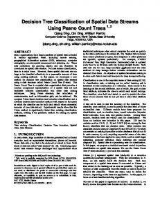
its characteristics like size, no. of rooms, garden size and so on. In data mining, a decision tree (it may be also called Classification Tree) is a predictive model that can be used to represent the classification model. Classification trees are useful as an exploratory technique and are commonly used in many fields such as finance, marketing, medicine and engineering [2, 3, 4, 5]. The use of decision trees is very popular in data mining due to its simplicity and transparency. Decision trees are usually represented graphically as a hierarchical structure that makes them easier to be interpreted than other techniques. This structure mainly contains a starting node (called root) and group of branches (conditions) that lead to other nodes until we reach leaf node that contain final decision of this route. The decision tree is a self-explanatory model because its representation is very simple. Each internal node test an attribute while each branch corresponds to attribute value (or range of values). Finally each lead assigns a classification. Fig. 1 shows an example for a simple decision tree for “Play Tennis” classification. It simply decides whether to play tennis or not (i.e. classes are Yes or No) based on three weather attributes which are outlook, wind and humidity [6]. Outlook Sunny

Overcast

Rain

YES Humidity

Wind Normal

NO

YES

Strong

Weak

NO

YES

Figure 1. Decision Tree Example.

As shown in Fig. 1, if we have a new pattern with attributes outlook is “Rain” and wind is “Strong”, we shall decide not to play tennis because the route starting from the root node will end up with a decision leaf with “NO” class.

17 | P a g e www.ijacsa.thesai.org

(IJACSA) International Journal of Advanced Computer Science and Applications, Vol. 3, No. 10, 2012

In this paper, we introduce a supervised learning technique of building a decision tree model for King Abdulaziz University (KAU) admission system to provide a filtering tool to improve the efficiency and effectiveness of the admissionprocess.KAU admission system contains a database of records that represent applicant student information and his/her status of being rejected or accepted to be enrolled in the university. Analysis of these records is required to define the relationship between applicant’s data and the final enrollment status. This paper is organized into five sections. In section 2, the decision tree model is presented. Section 3 provides brief details about commonly used methods for classification model evaluation. In section 4, experimental results are presented and analyzed with respect to model results and admission system perspective. Finally, the conclusions of this work are presented in Section 5. II.

B. Splitting Criterion ID3 algorithm uses some splitting criterion function to select the best attribute to split with. In order to define this criterion, we need first to define entropy index that measures the degree of impurity of the certain labeled dataset. For a given labeled dataset S with some examples that have n (target values) classes {c1, c2, …, cn), we define entropy index (E) as in (1). n

S ci

i 1

S

E (S )   p i *log( p i ), p i 

(1)

Where S ci the subset of the examples that have a target value that equals to c i . Entropy (E) has its maximum value if all the classes have equal probability. ID 3(S , F , c , SC )

DECISION TREE MODEL

A decision tree is a classifier expressed as a recursive partition of the input space based on the values of the attributes. As stated earlier, each internal node splits the instance space into two or more sub-spaces according to certain function of the input attribute values. Each leaf is assigned to one class that represents the most appropriate or frequent target value. Instances are classified by traversing the tree from the root node down to a leaf according to the outcome of the test nodes along this path. Each path can be transformed then into a rule by joining the tests along this path. For example, one of the paths in Fig. 1 can be transformed into the rule: “If Outlook is Sunny and Humidity is Normal then we can play tennis”. The resulting rules are used to explain or understand the system well. There are many algorithms proposed for learning decision tree from a given data set, but we will use ID3 algorithm due to its simplicity for implementation. In this section we will discuss ID3 algorithm for decision tree construction and some of the frequently used functions used for splitting the input space. A. ID3 Algorithm ID3 is a simple decision tree learning algorithm developed by Quinlan [7]. It simply uses top-down, greedy search over the set of input attributes to be tested at every tree node. The attribute that has the best split, according to the splitting criteria function discussed later, is used to create the current node. This process is repeated at every node until one of the following conditions is met: 

Every attribute is included along this path.



Current training examples in this node have the same target value.

Fig.2 shows the pseudo code for ID3 algorithm to construct a decision tree over a training set (S ) , input feature set (F ) , target feature (c ) and some split criterion (SC ) .

Output: Decision Tree T Create a new tree T with a single root node IF no more split (S) THEN Mark T as a leaf with the most common value of c a label. ELSE f i  F find f that has best SC (f i , S ) Label t with f FOR each value v j of f Set Subtree j  ID 3(S f

v j

, F  {f }, c , SC )

Connect node t to Subtree j with edge labeled v j END END Return T Figure 2. ID3 Algorithm

1) Information Gain To select the best attribute for splitting of certain node, we can use information gain measure, Gain (S, A) of an attribute A, bya set of examples S. Information gain is defined as in (2).

Gain (S , A )  E (S ) 



v V ( A )

S A v S

E (S A v )

(2)

Where E(S) is the entropy index for dataset S, V(A) is the set of all values for attribute A. 2) Gain Ratio Another measure can be used as a splitting criterion which is gain ratio. It is simply the ratio between information gain value Gain(S, A) and another value which is split information SInfo(S, A) that is defined as in (3).

SInfo (S , A ) 



v V ( A )

S A v S

*log

S A v S

(3)

3) Relief Algorithm Kira and Rendell proposed the original Relief algorithm to estimate the quality of attributes according to how well their values distinguish between examples that are near to each

18 | P a g e www.ijacsa.thesai.org

(IJACSA) International Journal of Advanced Computer Science and Applications, Vol. 3, No. 10, 2012

other [8]. The algorithm steps are stated in Fig. 3, where diff function calculates the difference between the same attribute value (A) within two different instances I1 and I2 as in (4).

0 diff (A , I 1 , I 2 )   1

I 1[ A ]  I 2 [ A ]



Recall (R) and Precision (P) are measures that are based on confusion matrix data. Recall (R) is the portion of instances that have true positive class and are predicted as positive. On the other hand, Precision (P) is the probability of that a positive prediction is correct as shown in (6).

otherwise

R

Relief Input: Training set S with N examples and K attributes Output: Weights vector W for all attributes A Set all weights W [1..K ]  0 FOR i = 1 to N Select random example R. Find nearest hit H (instance of the same class). Find nearest miss M (instance of different class). FOR A = 1 to K diff (A , R , H ) diff (A , R , M ) W [ A ] W [ A ]   N N END END Return W Figure 3. Relief Algorithm

III.

MODEL EVALUATION

Consider a binary class problem (i.e. has only two classes: positive and negative), the output data of a classification model are the counts of correct and incorrect instances with respect to their previously known class. These counts are plotted in the confusion matrix as shown in table 1. TABLE I. True Class Positive Negative

CN CP N

As shown in table 1, TP (True Positives) is the number of instances that correctly predicted as positive class. FP (False Positives) represents instances predicted as positive while their true class is negative. The same applies for TN (True Negatives) and FN (False Negatives). The row totals, CN and CP, represent the number of true negative and positive instances and the column totals, RN and RP, are the number of predicted negative and positive instances respectively. Finally, N is the total number of instances in the dataset. There are many evaluation measures used to evaluate the performance of the classifier based on its confusion matrix resulted from testing. We will describe in more details some of the commonly used measures to be used later in our experiment. Classification Accuracy (Acc) is the most used measure that evaluates the effectiveness of a classifier by its percentage of correctly predicted instances as in (5). Acc 

TP TN N



(6)

Precision and recall can be combined together to formulate another measure called “F-measure” as shown in (7). A constant  is used to control the trade-off between the recall and the precision values. The most commonly used value for  is 1 that represents F1 measure.

F 

(1   2 ) * P * R ( 2 * P )  R

(7)

For all the defined measures above, their values range from 0 to 1. For a good classifier, the value of each measure should reach 1. Another common evaluation measure for binary classification problems is ROC curve that is firstly proposed by Bradley in [9]. It is simply a graph that plots the relation between the false positive rate (x-axis) and true positive rate (y-axis) for different possible cut-points of a diagnostic test. The curve is interpreted as follows: 

The closer the curve follows the left-hand border and then the top border of the ROC space, the more accurate the test.



The closed the curve comes to the 45o diagonal of the ROC space, the less accurate the test.



The area under the ROC curve measures overall accuracy. An area of 1 represents a perfect test, while an area of 0.5 represents a worthless test.

CONFUSION MATRIX (BINARY CLASS PROBLEM) Predicated Class Positive Negative TP FN FP TN RN RP

TP TP and P  CN RN

IV.

EXPERIMENTS

A. Dataset King Abdulaziz University (KAU) admission system in the Kingdom of Saudi Arabia (KSA) is a complex decision process that goes beyond simply matching test scores and admission requirements because of many reasons. First, the university has many branches in KSA for both division male and female students. Second, the number of applicants in each year is a huge which needs a complex selection criterion that depends on high school grades and applicant region/city. In this paper, we are provided by sample datasets from KAU system database that represent applicant student information and his/her status of being rejected or accepted to be enrolled in the university in three consecutive years (2010, 2011 and 2012). The dataset contains about 80262 records, while each record represents an instance with 4 attributes and the class attribute with two values: Rejected and Accepted. The classes are distributed as 53% of the total records for “Rejected” and 47% for “Accepted” class. Table 2 shows detailed information about datasets attributes.

19 | P a g e www.ijacsa.thesai.org

(IJACSA) International Journal of Advanced Computer Science and Applications, Vol. 3, No. 10, 2012

The dataset is divided into two main parts: training dataset that holds about 51206 records (about 64%) and testing dataset that contains about 29056 records (about 36%). The decision tree classifier is learnt using a training dataset and its performance is measured on not-seen-before testing datasets. TABLE II.

SUMMARY OF DATASET ATTRIBUTES

Attribute Gender

Possible values Student’s gender

 Male  Female Type of high school study  TS = Scientific Study  TL = Literature Study  TU = Unknown/Missing High school grade  A = mark ≥ 85  B = 75 ≥ mark > 85  C = 65 ≥ mark > 75  D = 50 ≥ mark > 65 Code for student’s region city (116 distinct value)

HS_Type

HS_Grade

Area

C. Decision Tree Induced Rules1 One of the main advantages of the decision tree is that it can be interpreted as a set of rules. These rules are generated by traversing the tree starting from the root node till we reach some decision at a leaf. These rules also give a clear analytical view of the system under investigation. In our case, they will help KAU admission system office to understand the overall process. The induced set of rules is stated in table 5. TABLE V. DECISION TREE RULES SET

B. Decision Tree Model Results The decision tree model is generated over training dataset records using Orange data mining tool [10]. The generated decision tree is a binary tree with “One value against others” option. The confusion matrix valuesare shown in table 3. The values of confusion matrix are generated by applying a decision tree on testing datasets. TABLE III. True Class Accepted Rejected

Predicated Class Rejected 1538 6729 8267

13843 15213 29056

TABLE IV. MODEL EVALUATION MEASURES MeasureValue Accuracy Acc  R Accepted 

Recall R Rejected 

12305  6729 29056

12305 13843 6729 15213

PAccepted 

Precision PRejected

 0.442

F 1Rejected 

0.592  0.889 2 * 0.834 * 0.442 0.834  0.442

IF Area ≠ ”1007” AND HS_Grade ≠ ”A” AND HS_Grade ≠ ”B” THEN “Rejected” (98.9%) IF Area ≠ ”1007” AND HS_Grade = ”A” AND Gender = ”Male” AND Area ≠ ”1001” THEN “Rejected” (51.1%)

IF Area = ”1007” AND HS_Grade ≠ ”A” AND HS_Grade = ”B” THEN “Rejected” (63.9%)

 0.592 20789 6729   0.834 8267

F1 Measure

IF Area ≠ ”1007” AND HS_Grade = ”A” AND Gender = ”Female” AND Area ≠ ”901” THEN “Rejected” (64.4%)

IF Area = ”1007” AND HS_Grade ≠ ”A” AND HS_Grade ≠ ”B” THEN “Rejected” (87.0%)

 0.889

2 * 0.592 * 0.889

IF Area ≠ ”1007” AND HS_Grade = ”A” AND Gender = ”Male” AND Area = ”1001” THEN “Accepted” (74.9%)

IF Area ≠ ”1007” AND HS_Grade ≠ ”A” AND HS_Grade = ”B” THEN “Rejected” (90.5%)

 0.655

12305

F 1Accepted 

IF Area = ”1007” AND HS_Grade = ”A” THEN “Accepted” (75.7%)

IF Area ≠ ”1007” AND HS_Grade = ”A” AND Gender = ”Female” AND Area = ”901” THEN “Rejected” (85.0%)

TESTING CONFUSION MATRIX Accepted 12305 8484 20789

admission staffs can focus their energy on the most promising candidates to make a better selection. So, the workload on the administrative staff is much reduced and hence they may be able to make a better selection job. In fact missing some (i.e., With a recall slightly lower than 1) is not necessarily bad, as the administrative staffs may not always be able to identify the best candidates from a large pool. On the other hand, the same measures in case of “Rejected” class are about 0.58. This midlevel value stated that the classifier performance is above average.

As shown in table 5, beside each rule there is the percentage of instances that have the predicted class by this rule. Also, we can figure out that there are only two rules that lead to “Accepted” state. The first occurs if the student area code is “1007” (which is “Jeddah” city) and student’s high school grade is “A” (which is excellent student). The second case when “Male” student from area with code “1001” (which is “Rabigh” city) with grade “A” in high school.

 0.711  0.578

The evaluation measures shown in table 4 shows that the proposed classifier achieved a high recall at the cost of moderate precision. This means that a filtering tool improved the efficiency and effectiveness of the admission process. The classifier is to filter out the low level candidates so the

V.

CONCLUSION

In this paper we presented an efficient classification model using decision tree for KAU university admission office. The experimental results show that a filtering tool improved the efficiency and effectiveness of the admission process. This is

20 | P a g e www.ijacsa.thesai.org

(IJACSA) International Journal of Advanced Computer Science and Applications, Vol. 3, No. 10, 2012

achieved by the decision tree classifier with high recall under moderate precision (which determines the candidate pool size).we induced a set of rules by using the decision tree structure that helps KAU admission officeto make a better selection in the future. The model stated that the most accepted students from “Jeddah” region in KSA with excellent high school grade (more than 85%) or male students from “Rabigh”. REFERENCES [1] [2]

[3]

J. Han and M. Kamber, (2000),“ Data mining:concepts and techniques“, San Francisco, Morgan-Kaufma. H.S. OH and W.S. SEO, (2012), “Development of a Decision Tree Analysis model that predicts recovery from acute brain injury“, Japan Journal of Nursing Science. doi: 10.1111/j.1742-7924.2012.00215.x G. Zhou and L. Wang, (2012), “Co-location decision tree for enhancing decision-making of pavement maintenance and rehabilitation“,

Transportation Research: Part C, 21(1), 287-305. doi:10.1016/j.trc.2011.10.007 [4] S. Sohn and J. Kim, (2012). “Decision tree-based technology credit scoring for start-up firms: Korean case “, Expert Systems With Applications, vol. 39(4), 4007-4012. doi:10.1016/j.eswa.2011.09.075 [5] J. Choand P.U. Kurup, (2011), “Decision tree approach for classification and dimensionality reduction of electronic nose data“, Sensors & Actuators B: Chemical, vol. 160(1), 542-548. [6] T. Mitchel, (1997), Machine Learning, USA, McGraw Hill. [7] J. R. Quinlan, (1986), “Introduction of Decision Tree”, Machine Learning, vol. 1, pp. 86-106. [8] K. Kira and L.A. Rendell (1992), “A practical approach to feature selection”, In D.Sleeman and P.Edwards, editors, Proceedings of International Conference on Machine Learning, pp. 249-256, Morgan Kaufmann. [9] A.P. Bradley, (1997), “The use of the area under the roc curve in the evaluation of machine learning algorithms”, Pattern Recognition, vol. 30, pp. 1145-1159. [10] Orange Data Mining Tool: http://orange.biolab.si/

21 | P a g e www.ijacsa.thesai.org