recently edited Active Vision with Alan Yuille (MIT Press). He currently serves ... of neural networks, including a book (co-authored with Dr. Alan Murray of.
IEEE TRANSACTIONS ON ROBOTICS AND AUTOMATION. VOL. 1 I , NO 5, OCTOBER 1995
625
A Design for a Visual Motion Transducer Andrew Blake, Member, IEEE, Gabriel Hamid, and Lionel Tarassenko
Abstract -Autonomous vehicles could benefit greatly from visual-motion sensors of sufficientlylow cost that 10 or 20 of them could be distributed around the vehicle’s periphery. Conventional arrangements with CCD cameras, framestores and computers are too expensive. A design is outlined here that builds on well-known schemes using gratings. The grating principle is illustrated by the fact that a man with a torch, walking at night behind a railing, seems to flash. The frequency of flashing is proportional to his velocity. A major drawback is that backward and forward motion are not distinguished. The key development here is the use of commutation as a means of modulating the grating output signal. This is equivalent, in the illustration above, to simulating stroboscopic motion of the railing. Thus, when the man is stationary, there is flashing at a resting frequency. When he moves one way the frequency increases, and for motion the opposite way, frequency decreases. Results from an analogue implementation of the visual motion transducer are presented. The current transducer measures translational motion across the grating. The design is also shown to be capable of extension to direct measurement of the divergence and curl of the flow field.
lens
grating
, al plane
/
photodetector
I. INTRODUCTION
T
HE principle of grating Transducers has been outlined in papers by Ator [3], Agar [2], Gardner [8], and more recently by Itakura [14] and Yamasaki [20], [19]. Note that the term grating is not to be taken to imply coherent optical processing, for instance using a Fourier Transform plane [lo]. The gratings used are coarse graticules at spatial frequencies of several lines per millimeter. The grating sensor differs fundamentally from those based on correlation (Franceschini et al. [7]) in that it acts directly in the spatio-temporal frequency domain. Models of visual motion measurement developed for television camera sensors have also been based on the correlation idea or variants using spatio-temporal differential operators [ 121. The principles have been successfully integrated into the “silicon retina” [ 131 which produces an array of motion signals by analogue means. In contrast, the grating transducer is driven directly by a simple photodetector, rather than a camera, produces only one motion signal rather than an array of them and, being free of any frame synchonization requirements, can operate at far higher temporal bandwidths than a camera-based system. The grating transducer is an analogue device giving a direct reading of velocity coded as the frequency of the output signal. In this respect it differs from the approach of Buxton and Manuscript received November 13, 1992; revised August 10, 1994. The authors are with the Department of Engineering Science. University of Oxford, Oxford OX1 3PJ, U.K. IEEE Log Number 9409729.
Fig. 1. The basic grating sensor consists of an optical system imaging a scene through a grating, onto a photodetector. Both grating and photodetector are in the focal plane. Sensor output is thus proportional, at a given instant, to the total image irradiance summed over the transparent bars of the grating. Note that the sensor measures the motion of the whole of the imaged-scene. The grating and photosensor combination may, in practice, be an array whose photosensitive elements correspond to the transparent elements of the grating.
Buxton [5] which requires edge features to be detected in the output of a spatio-temporal Laplacian operator. It also differs from Heeger’s [ 111, [ l ] bank of spatio-temporal Gabor filters whose outputs must then be combined into a (least-squares) estimator for the velocity of a hypothesized moving plane. In the following section two explanations are given for the operation of the conventional grating transducer design. One explanation is algebraic, in terms of signal processing theory. The other is graphical, illustrating filtering operations in the spatio-temporal frequency domain. That sets up the computational framework for the key idea of the paper4ommutation. 11. THE GRATINGPRINCIPLE
A schematic diagram of the sensor is shown in Fig. 1. To explain the operation of the grating transducer, we introduce the following notation. We use (x,t ) (x,y, t ) for spatio-temporal coordinates and their duals in the frequency domain are (k, w) ( I C , I , w).The intensity distribution in the focal plane, just before the grating, is f(x,t)-this is simply the imaged scene, and its spatio-temporal Fourier transform is F ( k ,U ) . The grating is modeled by its transmissivity function g(x,t)and its Fourier Transform G. The output signal s ( t )
1042-296)(/95$04.00 0 1995 IEEE
626
IEEE TRANSACTIONS ON ROBOTICS AND AUTOMATION, VOL. 11, NO. 5, OCTOBER 1995
from the grating transducer is the result of multiplying the grating by the image signal, followed by spatial integration:
J 9(x, t)f(x,t)d2X,
s(t> =
spectrum F of moving image lies on inclined plane in w-k space
W
(1)
where the integration is over the infinite x-plane. A. Uniform Motion
In the case of uniform 2-D image-motion with velocity v,
f has the special form f ( x , t) = 7 ( x - vt)
so that its spectral distribution is confined to a plane [ 111: F(k,w) = F(k)S(w
+ k*v),
where is the spatial Fourier Transform of 7 and S is the Dirac delta-function. In the normal case that the grating is static (relative to the optical system) then
Fig. 2. The action of the basic grating transducer is pictured here in the frequency domain. Since the grating is static, its transfer function lies within the k plane. Assuming uniform image motion, the w - k spectrum F of the image intensity distribution lies on an inclined plane. The gradient of the plane is the image velocity v. The action of the grating transfer function is to pick out certain components of F and map them onto the w axis where they sum to produce the transducer output.
B. Infinite Grating Model We will consider an idealized grating, one of infinite extent,’ whose MTF has the form
n
where ko is the vector wavenumber (in lines/”) of the fundamental component of the grating transmissivity function 9. Substituting this into the slice relation (4)we obtain
and
G(k,w) = G(k)S(w).
1
c
Note that is simply the MTl-the spatial Transfer Function-that describes the effect of the grating within the optical system. With these assumptions, the formula (1) simplifies to
J
~ ( t=) ~ J ( x ) ~ (-x vt)d2x, which strongly resembles a spatial convolution integral. Denoting spatial convolution by *, (2) can be written simply as
where ij is the reflection of ij defined by j(x)
S(W)= 2.rr
c Z S ( n ~ o- w)F(nko)
(6)
n
where
Thus the signal s ( t ) consists of a dc component and harmonics of the fundamental frequency W O . The fundamentalfrequency of the transducer output is therefore directly proportional to the vector component of image motion v orthogonal to the grating bars. The amplitude of the fundamental is proportional to the spectral content F(k0) of the image signal at the corresponding spatial frequency. Provided the image signal does not have a gap in its spectrum at that point (e.g., a grey, featureless plane) a measurable fundamental should be obtained.
iJ(-x).
C. A k - w Space Explanation The corresponding relation in the frequency domain is
An alternative explanation of the action of the Transducer can be given in the three-dimensional k - w space and this S(w) = 2n /G*(k)F(k)S(k.v w ) d2k. (4) is illustrated in Fig. 2. An advantage of this explanation is that it readily extends to explain intuitively the commutation effect described below. The idea is that the Transducer output This is a summed slice, orthogonal to the velocity vector v, signal consists of spectral components S(w) that are obtained through the product of signal spectrum F and grating transfer simply by superimposing G and F. The justification for this function G (where denotes the complex conjugate). It is simply the dual of the slicing operation that occurs in axial effect of truncating the grating to a finite extent is to cause a transmission tomography 141. broadening of its spectral lines [lo].
+
c*
621
BLAKE et al.: VISUAL. MOTION TRANSDUCER
1.o
__x
08 0.6 0.4
0.2 -0 0
I T
140
-0.2
160
-0.4 -0.6
-0.8 -1.o -1.2
j
Fig. 3. The operation of existing designs of grating Transducer is illustrated. An Adept robot carries a CCD camera slowly (4 m d s ) across the scene in Fig. 4 and then stops. The differential grating sensor of Fig. 1 is simulated in software. Note that for a sensor with a differential grating there is no dc signal level when the sensor is moving. (Horizontal axis: camera frames, rate 25 framesk Vertical axis: arbitrary units.)
is as follows. From ( I ) and using the dual of the convolution theorem:
where Z(k,w)=G*F.
(9)
(Note that here * denotes 3-D convolution in w - k space.) Hence S ( w ) is computed by sliding G through a distance w along the vertical axis in Fig. 2 and superimposing it (i.e., multiplying and summing) onto F . Clearly, the center frequency WO of the output spectrum is proportional both to magnitude of velocity v (gradient of the F-plane) and the spatial frequency lkol of the grating. This is consistent with the algebraically derived relation (7) above. For simplicity, in the case illustrated, only the fundamental component of the transmissivity of the grating is shown and this produces just one spectral component (or, in practice, a narrow packet) in the output S ( w ) . Including a dc component and higher harmonics would simply produce, by the superimposition process, a temporal dc component and higher harmonics in the output. The dc component is a serious nuisance as it tends to swamp the desired fundamental. It can be attenuated however by more sophisticated “differential” grating arrangements and by high-pass filtering [8]. Fig. 3 shows a typical signal from a simulation using a differential grating. The higher harmonics are naturally less problematic because they tend to be weaker in the grating’s transfer function ?%harmonics of a square wave grating, for instance, fall off in inverse proportion with frequency. Higher harmonics also tend to be weaker in the scene spectrum F. For a typical fractal scene, harmonic amplitude decays with frequency at rate between lkl-1/2 and lkl-3/2 [16].
111. LIMITATIONS OF EXISTINGANALOGUE DESIGNS There are two problems with the basic grating sensor. I ) It does not relay the sign of velocity, that is one cannot distinguish, from the sensor output, between forward and
Fig. 4. This image shows the scene used in simulations. Robot motion is arranged such that a simulated grating in a roughly square window NnS from top to bottom of the image shown.
backward motion. This is because sidebands occur in symmetrical pairs (6). 2) At zero velocity, the frequency of the sensor signal falls to zero, as shown in the simulation of Fig. 3. This is highly inconvenient for hardware implementation as dc amplifiers must be used and very low frequencies must be measured to operate at near-zero velocities. The two problems above would be removed if somehow an artificial motion of the grating could be induced. In that case, the induced velocity 710 of the grating would add to the component 11 of real motion to produce a fundamental frequency proportional to WO w. That has the effect of moving the center frequency of the system up from 0 to s1 = wolkol which can be as high as convenient for hardware purposes. (Operating in an ac mode is a common hardware technique for circumventing low frequency noise sources.) Furthermore, the fundamental frequency is increased by forward motion and decreased by reverse motion. Now the sign of velocity can be distinguished.
+
Iv. EXISTINGDESIGNSFOR ARTIFICIAL MOTIONOF THE GRATING Itakura [ 141 constructs a physically moving grating using Liquid Crystal Display technology. The grating is constrained to move in discrete jumps due to the finite number of liquid crystal cells. The intermittent movement of the grating causes broadening of the motion signal frequency spectrum. Broadening of the frequency spectrum increases the uncertainty in the velocity measurement, i.e., reduces accuracy. A stationary sinusoidal grating has the form cos(z). A laterally moving sinusoidal grating has the form cos(z u t ) , which can be expanded as:
+
cos(n:
+ ut) = cos z cos v t - sin z sin wt.
(IO)
IEEE TRANSACTIONS ON ROBOTICS AND AUTOMATION, VOL. 11, NO. 5, OCTOBER 1995
628
0.6 0.4
I
I
I
I
0.2
It)
0.0
Fig. 5. Three-phase grating. Each period (of length 27r/lkoI) of the conventional grating of Fig. 1 is subdivided into three phases. This can be achieved by using a multielement photo-sensitive array, as shown. Three signals are constructed by summing signals from elements labeled 1, 2, 3 respectively. Commutation between the three signals should, intuitively, generate an artificial "stroboscopic" motion in the grating plane.
Hence, the moving grating can be constructed from two spatial filters in quadrature and two oscillators in quadrature. Yamasaki [19] has implemented this approach, using a signal generator to weight the output of a video camera. The next section describes the commutation idea, which leads to a simple analogue implementation.
1
160
-0.2 -0.4
-0.6
4
-0.8
Fig. 6. Velocity transducer using commutation. The simulated signal output is shown for backward motion followed by stasis. The output consists of an interval at lowered frequency followed by an interval at the commutation frequency. Compare with the output of the conventional grating sensor, in Fig. 3, for the same motion sequence. Results shown are for a six phase (A4= 6) system. (Horizontal axis: camera frames, rate 25 frameds.)
4
0.8 0.6 0.4
v.
STROBOSCOPIC MOTIONINDUCED BY COMMUTATION
Artificial motion of the grating can be induced by subdividing the grating cycle into M phases, as in Fig. 5 . The sensor now generates several outputs s o ( t ) ?s l ( t ) ,. . . ,s M - l ( t ) . In the case illustrated M = 3 and this is the minimum for the commutation idea to work. The combined output s ( t ) is produced by commutation between the phases at a frequency
0.2 0.0 -0.2 -0.4
-0.6
-1.0 -o'8
R: M
cos(Rt - 27rm/M)s,(t).
s(t) =
(11)
m=O
It is clear that, in the absence of real motion, when s m ( t ) are constants, s ( t ) is oscillatory with fundamental frequency R. This is already promising since one of our goals is to have a nonzero fundamental frequency at zero velocity. That would be the case even in the absence of the multiplicative cosine weightings. The weightings are included to ensure correct additive behavior for sensed velocity without creating spurious higher temporal harmonics. Simulation of the conventional grating sensor, done with a CCD camera mounted on a moving robot, was shown earlier in Fig. 3. Now the simulation is repeated for the new Transducer that employs commutation (Figs. 6 and 7). As claimed, and shown theoretically below, a signal of frequency R is generated when the scene is stationary. For forward motion, sidebands are generated and the frequency of the fundamental is greater than 0.For reverse motion the frequency of the fundamental falls below R. Simulation here is for a six-phase (M = 6) system which means, as shown in a later analysis that the 2nd, 3rd, and 4th harmonics are suppressed. Hence the fundamental frequency shows up clearly in Fig. 6 and zero-crossing counting is more or less adequate as a means of frequency measurement.
1
'
Fig. 7. Velocity transducer using commutation. As Fig. 6 but now for forward motion followed by stasis. Signal frequency is elevated during the forward motion. (Horizontal axis: camera frames, rate 25 frameds.) Note that the amplitude of the signal depends upon the amount of spatial intensity variation in the imaged-scene, so that when the scene is well-textured the amplitude of the signal is large, but when the scene is fairly featureless, the amplitude of the signal is small.
A. The k - w Space Explanation The k - w space explanation for the conventional grating sensor can be extended now for commutation. The commutation induces artificial grating motion-this is, in principle, a standard stroboscopic effect. The picture of Fig. 2 must therefore be modified. If the whole of the grating was moving, then the spatio-temporal pass-band G of the grating would lie not on the k-plane but on an inclined plane with a gradient equal to the velocity of the induced motion. The effect of commutation is slightly different, Hamid [9] has shown that the effect of commutation is to shift the plane containing the transfer function G of the grating, to the two planes (U( = R. Fig. 8 shows that, using the previous superposition construction, the effect is to displace the spectrum of the output signal (on the w-axis) by R. The frequency of the first harmonic is now R k0.v.
+
B. Commutation as a Modulation Effect An alternative to the k - w space view is to treat the commutation as a form of signal modulation. In the basic
629
BLAKE et al.: VISUAL MOTION TRANSDUCER
n
w ?
i
2
3
0
i
2
3
0
F of moving image lies on indinedplam in w k space
spec" Gensducer signal
\
Fig. 8. The effect of commutation in the frequency domain. Since the grating is now in stroboscopically induced motion, its transfer function lies on the planes lijl = (2 (compare with Fig. 2). This displaces the output signal spectrum along the G-axis (again, compare with Fig. 2).
sensor, the output is a series of harmonics (6) symmetrically positioned about 20 = 0. The effect of commutation is to apply a frequency shift so that the harmonics become sidebands of the commutation frequency R. Furthermore, and most importantly, one sideband of each harmonic pair is suppressed. The remaining sideband is above or below R according to whether the motion is forward or backward. We now show this. Suppose the scene is in uniform image-motion with velocity v. Then the 0th phase of the sensor output can be expressed as a Fourier series
an exp(in.ko.vt).
so@)=
Other phases are simply delayed versions of the 0th:
an cxp(inko.vt) exp(-27rinm/M).
(13)
n
After commutation (11) the combined signal is
s(t)=
nf
~ o n [ c x p i ( ( R + n k ~ ~ v ) t - 2 7mr - ( n + 1 ) )
M
m=O n
+exp-i
m, (R - nko.v)t - 2.rr-(n
(
M
-
I))]
(14)
which can be expressed as
=Mean[?(%)
~(t)
Frequency lo
signal voltage
velocity
Fig. 9. Motion transducer circuit. The photodiode array is organized into four phases by summation of signals from the array elements. The commutation oscillator generates a sinewave at frequency Q. The frequency-coded velocity is converted to a voltage output proportional to velocity.
pair of sidebands for the nth harmonic. Provided M 2 3, at least one sideband of each pair must vanish. In the case of the fundamental ( n = l), Q((n 1)/M) = Q ( 2 / M ) = 0 but Q ( ( n- l)/M) = Q(0) = 1. Thus the sideband at frequency R nk0.v vanishes, leaving the single sideband at frequency R - nko.v. Hence the sign of the velocity v can be detected from the frequency of the fundamental sideband. The intuitive argument given earlier clearly fails for M < 3 because stroboscopic motion will not occur for a system with only two phases. The algebra above is consistent here: in the case M = 2, for the fundamental frequency, Q((n+ 1)/M) = Q( 1) = 1 so both sidebands are present. Hence a two-phase system can, as expected, be used to remove dc but not to detect the sign of the velocity. Is there any point is choosing M > 3, given the extra complexity in the photodetector array and supporting electronics? In fact there is. In that case both sidebands disappear for 1 < n < M - 1. Increasing the number of phases in the grating beyond 3 causes some higher harmonics, up to the ( M - 2)th, to be suppressed.
+
+
n
s m ( t )=
signal frequency propoftlomi to velocity
expi(R+nko.v)t
n
+Q(?)
exp - i ( R - nko.v)t]
(15)
where
VI. HARDWARE VERSION A . Implementation
Q(t) =
{
1 if t is an integer 0 otherwise.
In the case that n = 0, assuming M 2 2 , we have Q(l/M) = Q(-1/M) = 0, so there is no dc term in (15). The dc component is suppressed by the commutation scheme. For n 2 0, the two exponential terms in (15) are the symmetrical
The elements of a linear photodiode array are subdivided into M phases. Any number of phases can be implemented by using the appropriate number of multiplier chips and an oscillator with the correct phase delays. However, using four phases enables a particularly neat implementation in analogue hardware. This can be seen by
630
IEEE TRANSACTIONS ON ROBOTICS AND AUTOMATION, VOL. 11, NO. 5, OCTOBER 1995
Power spectrum 20
-20
1
4
V 1150
Im
I250
1300
1350
1400
1450
I500
1550
1600
frequency (Hz)
Power spectrum 20 1816 14 12 -
10864-
2,
1150
1200
1250
1300
1350
1400
1450
I500
I550
16fM
frequency (Hz) Fig. 11. Power spectra of real sensor signal;. Here, the commutation frequency is at 1372 Hz. The top graph is for backward motion and the bottom graph for forward motion. The square root of the power spectrum has been used to reveal more detail.
Fig. 10. Typical frequency outputs from a real motion sensor. The three graphs show output voltage (units mV) against time (units s) of typical input signals to the zero-crossing counter of the velocity transducer. The top graph was recorded during backward motion, the middle graph from stasis and the bottom graph from forward motion. Note that for this figure we have deliberately slowed down the commutation frequency so that the motion-induced shifts in the frequency of the signals can be seen in the time domain. Usually the commutation frequency is much greater than the largest expected motion-shift in frequency.
writing out (1 1) fully for the case M = 4:
s ( t ) =s1(t) cosat + s 2 ( t )cos(Rt - 2)+ S 3 ( t ) cos(Rt - R) R
+
S4(t)
3R cos(Rt - -) 2
(16)
which reduces to: s ( t ) = [ S l ( t ) - S Q ( t ) ] cos R t
R + [ s z ( t )- s q ( t ) ] . cos(Rt - -).
?I71 Only one quadrature oscillator is required as shown in a schematic of the hardware in Fig. 9. The subtractions [ s l ( t )5 3 ( t ) ]and [s2 (t)-s4( t ) ]are implemented with instrumentation amplifiers to provide a high common-mode rejection.
B. Results Fig. 10 shows the motion transducer signal before frequency demodulation for stationary, forward and backward motion. Fig. 11 shows the Discrete Fourier Transform of typical motion transducer signals before frequency demodulation. Fig. 13 shows the variation of output frequency of the motion transducer with relative angular velocity to a textured surface.
Fig. 12 shows a sample of typical textured surfaces the sensor has been tested on. Fig. 14 shows the variaion of the accuracy of the sensor over its velocity range. All these results were obtained using normal indoor lighting. The signal to noise ratio (SNR) is high enough to allow frequency measurement to be performed by a zero-crossing counter. For high S N R the accuracy of the transducer is determined by the observation time and the width and shape of the frequency spectrum of the signal, see Schultheiss [18]. The width of the frequency spectrum decreases with the number of elements in the grating. Our current set up uses a photodiode array having 48 elements. A Hanning window changes the sinc shape of the frequency spectrum to a more Gaussian shape, as shown in Fig. 15, this improves the accuracy of the transducer. To mimic the effect of a Hanning window the width of the grating elements are varied, with narrower elements at the ends of the grating and wider elements toward the middle of the grating. A complete description of the design of the velocity sensor, including the compromises involved in choosing the grating structure for the best possible accuracy, can be found in [9].
VII. DEVELOPMENTS OF THE IDEA This last section describes how a family of transducers can be built, each of which is sensitive to one and only one component of the parallax field, the spatial derivative of the optic flow-field (Koenderink and van Doorn [15]). For instance a divergence detector can be fabricated by arranging the elements of the grating in concentric circles, as in Fig. 16. A curl detector can be fabricated by arranging the elements of the grating in radial segments around a ring, also shown in Fig. 16. Mitsuhashi [17] proposed the same circular and radial gratings for the video-based sensor described by Yamasaki
63 1
BLAKE et al.: VISUAL MOTION TRANSDUCER
Fig. 12. A diversity of textures, some of which are shown here, have been used to test the implementation of the analogue motion sensor.
[19], although of course circles cannot be defined accurately on a CCD array in the way that they can with customized photodiodes, as we propose. More importantly, whilst any reasonable design based on concentric rings will respond to divergence, it turns out that it is much more difficult to make a detector that responds only to divergence, rejecting other flow-field and parallax field components. This works only if the signal from the circular grating is processed in a particular way, described below, and a similar result is true for radial gratings and the curl component. Cipolla and Blake [6] point out that, as a consequence of the divergence theorem of vector calculus, the divergence of the velocity field may be approximated as a contour integral divv =
‘f’
-
L
v.nd.9
Frequency (Hz)
8ol
-14
-18
-1.2
/
0.6
1.2
1.8
2.4
relative angular velocity (rad / s)
(18)
around a closed contour, where s is the arc-length parameter and L is the total length of the contour. Moreover, this quantity is “immune” to other components of the velocity and parallax fields, and a similar result holds for curl. If, for instance, the visual sensor were traveling toward a target, a divergence component would be generated. If also the target were moving laterally, orthogonally to the line of sight, an additional uniform component would appear in the flow-field, but would be filtered out by the contour integral above. Intuitively, uniform flow on one side of the contour
Fig. 13. Graph showing the linearity of the real sensor. Frequency was measured by a zero-crossing counter, with an observation time of 1.4 s. The commutation frequency (1372 Hz) has been subtracted from the frequency measurement. The sensor has a linear output for object motions less than 1.2 radians per second.
is cancelled, in the integral, by flow on the opposite side. The question now is, what signal analysis process, if any, will compute the equivalent of that contour integral?
IEEE TRANSACTIONS ON ROBOTICS AND AUTOMATION, VOL. 11, NO. 5, OCTOBER 1995
632
*”’”*
RMS error in velocity measurement (rad I s)
\
1.0 .
\ \ \
\
4
Ilr m
0.8
-
0.7
-
-
0.1 second
0.6
0.5
-
/
0.9
\
L /
/
0:4second
1.5
2.0
Fig. 16. Arrangement of grating elements for divergence and curl detectors. The grating elements are arranged in concentric circles for the divergence detector, and in radial segments for the curl detector.
0.2
-2.5
-2.0
-1.5
4 . 5
-1.0
0.0
0.5
1.0
2.5
Angular velocity (rad / s) Fig. 14. The absolute accuracy of the real sensor. Frequency was measured by a zerocrossing counter, with three different observation times, the longer the period of observation the more accurate the sensor. Note that the motion was kept uniform throughout the period of observation.
0.7
%m
{
0.7
o.611
VIII. CONCLUSION
-
The originality of this paper rests in the commutation idea. An analogue implementation has validated the principle and confirmed that a practical device can be built which is accurately linear in velocity. The motion transducer requires only inexpensive analogue circuitry. The ideas have been extended to divergence and curl detectors.
06 -
a5
05
detector will operate correctly, if an analogue circuit can be built which measures Z. A zero-crossing counter is a sufficient device for measuring the centroid of the power spectrum of a signal with a high signal to noise ratio (SNR) and a compact power spectral density. For signals with a low SNR and a broad power spectral density, a more sophisticated frequency measuring device is required, such as a tracking filter.
-
ACKNOWLEDGMENT The authors would like to thank the following people for their help: W. Mitsuhashi, D. Witt, D. Hamilton, M. Srinivasan, and M. Brownlow. REFERENCES Fig. 15. Graph showing the improvement in the signal frequency spectrum by using a Hanning window. The left graph shows the Fourier transform of the grating function without a Hanning window. The right graph shows the transform of the same grating but with a Hanning window.
In our case the contour is simply a circle defined by the grating (assumed to be a thin annulus). Locally, in the interval (s, s ds), the ring-grating responds to the normal component of motion w(s) = v(s)-n(s), generating a signal centred at frequency w(s) cc w ( s ) with power P(w)dw. If we assume that the spectral power density of the underlying visual signal is homogeneous then the total power delivered by the interval will be proportional to its area, so that:
+
P ( w ) d w 0: ds.
In that case the integral in (18) becomes divv
0:
/w(s)P(w)dw
(19)
which is simply the centroid Z of the power spectrum P(w). The conclusion is that the divergence (and similarly curl)
[l] E. H. Adelson and J. R. Bergen, “Spatio-temporal energy models for the perception of motion,” J. Opt. Soc. Am., vol. A2, no. 2, pp. 284-299, 1985. [2] W. 0. Agar, “An optical method of measuring transverse surface velocity,” J. Scientific Instruments, Series 2, vol. 1, pp. 25-28, 1966. [3] J. T. Ator, “Image-velocity sensing with parallel slit reticles,” J. Opt. Soc. Am., vol. 53, no. 12, 1963. [4] R. N. Bracewell, The Fourier Transform and Its Applications. New York McGraw-Hill, 1986. [5] B. F. Buxton and H. Buxton, “Monocular depth perception from optical flow by space time signal processing,” in Proc. Royal Society of London, vol. B 218, pp. 2 7 4 7 , 1983. [6] R. C. Cipolla and A. Blake, “Surface orientation and time to contact from image divergence and deformation,” in Proc. 2nd ECCV, 1992, pp. 187-202. [7] N. Francescini, J. Pichon, and C. Blanes, “Visual guidance of a mobile robot equipped with a network of self-motion sensors,” in Proc. SPIE, vol. 1195, pp. 44-53, 1989. [8] P. Gardner, “A new approach to the measurement of image velocity,” Royal Aircraft Establishment, Tech. Memo IR 125, 1972. [9] G. Hamid, “A design for a vision-based velocity sensor,” D.Phi1. dissertation, Oxford University, 1993. [lo] E. Hecht and A. Zajac, Optics. Reading, MA. Addison-Wesley, 1975. [ 111 D. Heeger, “Optical flow from spatiotemporal filters,” Int. J. Computer Vision, pp. 181-190, 1987. [12] B. K. P. Hom and B. G. Schunk, “Determining optical flow,” Artificial Intell., vol. 17, pp. 185-203, 1981.
BLAKE er ai.:VISUAL MOTION TRANSDUCER
J. Hutchinson, C. Koch, J. Luo, and C. Mead, “Computing motion using analog and binary resistive networks,” IEEE Computer, pp. 52-63, Mar. 1988. Y. Itakura, A. Sugimura, and S. Tsutsumi, “Amplitude-modulated reticle constructed by a liquid crystal cell array,” Appl. Opt., vol. 20, no. 16, pp. 2819-2826, 1981. J. J. Koenderink and A. J. Van Doom, “Invariant properties of the motion parallax field due to the movement of rigid bodies relative to an observer,” Optica Acta, vol. 22, no. 9, pp. 773-791, 1975. B. B. Mandelbrot, Fractals: form chance and dimension. San Francisco, CA: Freeman, 1977. W. Mitsuhashi, K. Oka, and H. Yamasaki, “Motion measurement of dynamic images by the use of spatial filter built by electronic circuits (in Japanese),” Trans. Society of Instrument and Control Engineers, vol. 24, no. 11, pp. 1-7, 1988. P. Schultheiss, C. Wogrin, and F. Zweig, “Short-time frequency measurement of narrow-band random signals by means of a zero counting process,” J. Appl. Phys., vol. 26, 1955. H. Yamasaki, K. Oka, and W. Mitsuhashi, “An adaptive intelligent velocity sensing system,’’ in IEEE Tech. Dig. Transducers ’87, 1987, pp. 137-142. H. Yamasaki, M. Shimokawa, and W. Mitsuhashi, “New structure for intelligent sensors,” in IEEE Tech. Dig. Transducers ’85, 1985, pp. 38-41.
Andrew Blake (M’86) was born in England in 1956. In 1977, he graduated from Trinity College, Cambridge, with the B.A. degree in mathematics and electrical sciences. After a year as a Kennedy Scholar at MIT and two years in the electronics industry, he studied for a doctorate degree at the University of Edinburgh which was awarded in 1983. Until 1987 he was a Lecturer at the University of Edinburgh and a Royal Society Research Fellow. He is currently on the faculty of the Robotics Research Group in the University of Oxford. His research interests are in Robot Vision and also in human visual psychophysics. He has published a number of papers in vision, a book with A. Zisserman (Visual Reconstruction, MIT Press), and recently edited Active Vision with Alan Yuille (MIT Press). He currently serves on the program committees of the International and European Conferences on Computer Vision and on the editorial boards of Vision Research, Image and Vision Computing and International Joumal of Computer Vision. I
633
Gabriel Hamid was bom in England in 1968. In 1990, he graduated from Magdalen College, Oxford, with the B.A. degree in engineering and computer science. He studied for the doctorate degree at the Robotics Research Group in Oxford until 1993. He is currently working at VLSI Vision Ltd. as a design engineer developing specialized electronic hardware for machine vision.
Lionel Tarassenko was bom in Paris in 1957. He received the B.A. degree in engineering science in 1978, and the D.Phil. degree in medical engineering in 1985, both from Oxford University. He holds the following degrees: M.A., D.Phil., M E E , and CEng. After graduating, he worked for an industrial research laboratory on the development of digital signal processing techniques, principally for speech coding. He returned to Oxford University at the end of 1981 to undertake research in medical signal processing. This was followed by another period in industry, during which he led a team designing real-time control systems for medical instrumentation. Since being appointed a University Lecturer in 1988, he has devoted most of his research effort to the development of artificial neural network techniques and their application to diagnostic systems, robotics and parallel architectures. He has 70 publications in all, mostly in the field of neural networks, including a book (co-authored with Dr. Alan Murray of the University of Edinburgh).