A Design Methodology and Environment for Interactive ... - CiteSeerX

A Design Methodology and Environment for Interactive Behavioral Synthesis Daniel D. Gajski*, Tadatoshi Ishii**, Viraphol Chaiyakul*, Hsiao-Ping Juan* and Tedd Hadley*

Technical Report #96-29 June 15, 1996 *Department of Information and Computer Science University of California, Irvine Irvine, CA 92697-3425, USA **Multimedia Engineering Laboratory Toshiba Corporation 70 Yanagi-cho, Saiwai-ku, Kawasaki, 210 Japan

Abstract

Due to recent increases in chip complexity, behavioral synthesis has become an important area of research and company interest. However, there has been market resistance to the automatic behavioral synthesis approach for two reasons. It often produces results inferior to manual designs, and it allows only minimal user control. To overcome these hurdles, we present a design methodology for human interaction in design synthesis, which, in contrast to the automatic synthesis approach, gives the human designer ne-grain control over synthesis tasks, and continually supplies feedback in the form of quality measures so that the user can make informed design-related decisions. To con rm the feasibility of the proposed design methodology and to demonstrate its power and exibility, we also present the Interactive Synthesis Environment (ISE), a working software environment comprising design views, quality measure feedback, and synthesis algorithms.

Contents 1 Introduction

3

2 Previous Work

5

3 Interactive Design Methodology

6

4 The Interactive Synthesis Environment: ISE

7

4.1 Behavioral Level : : : : : : : : : : : : : : : : : : : : : : : : : : : : : : : : : 4.2 Structural Level : : : : : : : : : : : : : : : : : : : : : : : : : : : : : : : : : : 4.3 Physical Level : : : : : : : : : : : : : : : : : : : : : : : : : : : : : : : : : : :

8 10 12

5 An Example

13

6 Conclusion

20

1

List of Figures 1 2 3 4 5 6 7 8 9 10 11 12 13

A typical design methodology of an automatic behavioral synthesis system A design methodology for interactive behavioral synthesis : : : : : : : : : : The design view, quality metrics, and tasks supported in ISE : : : : : : : : The state-actions table view : : : : : : : : : : : : : : : : : : : : : : : : : : The component selection and binding view : : : : : : : : : : : : : : : : : : The oorplan view : : : : : : : : : : : : : : : : : : : : : : : : : : : : : : : : The speci cation of the SRA example : : : : : : : : : : : : : : : : : : : : : The state-actions table of the SRA example : : : : : : : : : : : : : : : : : The design of the SRA example after splitting ST1 and allocation : : : : : The design of the SRA example after the rst re-allocation : : : : : : : : : The design of the SRA example after splitting ST1 and ST4 : : : : : : : : The design of the SRA example after binding : : : : : : : : : : : : : : : : : The design of the SRA example after the second re-allocation : : : : : : :

2

4 7 8 9 10 12 14 15 16 17 18 19 20

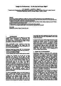
1 Introduction Recent advances in VLSI technology have allowed companies to build complex designs containing over one million transistors on a single chip. As the complexity of chips increases, so will the need for designing from the behavioral abstraction level where functionality and tradeos are easier to understand and control. Behavioral synthesis is a process of synthesizing a design from a given behavioral description to a register-transfer-level (RTL) structure. Behavioral descriptions can be programs, algorithms, owcharts, data ow graphs, instruction sets or generalized nite-state machines. The RTL structure is a set of interconnected components described as a netlist. Components in the netlist can be (a) functional units such as ALUs, multipliers, (b) storage units such as memories, register les, and (c) interconnection units such as muxes and buses. In general, behavioral synthesis involves three major tasks: allocation of physical resources (i.e., functional units, storage units and interconnection units) to be used in the design, scheduling of behavioral tasks into time intervals, and binding of behavioral operations and variables to physical resources. Many years of research have been devoted to the development of automatic behavioral synthesis systems [2][3][6][10]. In these systems, designs are obtained with minimal user interaction in that the only means of controlling the desired output is via the input description and via constraints expressed in terms of area and/or performance. Figure 1 shows the typical design methodology of an automatic behavioral synthesis system. Note that the order in which synthesis tasks are performed may vary. Automatic behavior synthesis suers from a number of complex issues.

 The synthesis tasks are all NP-complete problems and heuristics must be employed when brute-force approaches would take too much time to complete.

 The order in which synthesis tasks are performed has an impact on both the eciency and quality of results. Automatic systems usually have one xed order of tasks.

 The behavioral synthesis tasks are always done before the physical level tasks, such

as placement and routing. Yet, these low level tasks contribute signi cantly to the delay and area of the design and such eects are very dicult to estimate at the behavior level. Hence, resulting designs sometimes cannot satisfy the performance or 3

area demands of real-world constraints. Although it certainly cannot be denied that considerable progress has been made in this research area, a practical solution to automating behavioral synthesis is still distant. Start

Specify design behavior

Set constraints for synthesis system

Allocation

Scheduling

Automatic Behavioral Synthesis

Binding

Placement & Routing

no

Constraints met? yes End

Figure 1: A typical design methodology of an automatic behavioral synthesis system When the design produced by automatic behavioral synthesis is not a good one, the user is presented with the following dilemma. She may either modify the input description or constraints, which may result in yet another design which does not satisfy constraints, or modify the synthesized design manually, which requires considerable eort to understand, to manipulate and to verify that the changes made resulted in a correct design. To develop a feasible approach to behavioral synthesis, we have substituted the goal of a completely automated, \push-button" synthesis system with one which attempts to maximally utilize the human designer's insights. Using interactive behavioral synthesis, 4

the user can control the design process, observe the eects of design decisions, and manually override synthesis algorithms at will. This interactivity will allow a synthesis system to generate complex designs of acceptable quality in the immediate future instead of waiting the many years before current automatic synthesis techniques reach a similar level of quality. With this goal in mind, we have implemented a system called the Interactive Synthesis Environment (ISE) to demonstrate the feasibility of such methodology In the next section, we describe previous and comparable work in the area of interactive synthesis. Following that, we oer the proposed design methodology as a superior alternative to automatic synthesis methodology. We then introduce the interactive synthesis system ISE in Section 4 as a testable instantiation of our design methodology. Finally we present a walk-through design synthesis example and present our conclusions.

2 Previous Work There are several previous papers that address the importance of user-interaction with synthesis systems. In this section, we will dierentiate our approach from previous research. The ACE graphical interface [1] is intended to function between the user and the synthesis system. It allows the user to place and connect functional nodes to create graphs that specify the desired behavior, thereby precluding the need for an initial textual input description. After the initial graphical speci cation is obtained, and before synthesis tasks such as allocation, scheduling and binding start, transformation techniques can be applied by the user to the speci cation to change it into a better, more ecient input description of the synthesis system. ACE allows the user to interact with the synthesis system by giving the user the nal say in accepting or rejecting the system's transformation decisions. An experienced user can also specify transformations manually. Nevertheless, ACE does not allow the user to interact directly with the synthesis tasks. RLEXT [8] [9] is an interactive tool which allows a user to manually reschedule a design's behavior or modify a design's structure by adding or deleting components and interconnects. The unique aspect of RLEXT is that, if the user makes changes in the datapath design or the behavior's schedule that would impair the datapath's ability to carry out the desired schedule, RLEXT will automatically repair the datapath so that it is once again able to execute the speci ed schedule. However, RLEXT does not provide the user with feedback as to the current design's quality to assist the user in making subsequent design decisions. 5

The system AMICAL [7] allows the user to mix automatic and manual design. The user may start a design manually and ask AMICAL to nish it. Alternatively, the user can execute the synthesis tasks step by step. At each step, the user has the choice to continue the synthesis automatically or manually. However, AMICAL requires the user to follow a xed order of synthesis tasks. A unique aspect of our approach is that it allows the user to start oorplanning early in the design process. None of the previous research addresses physical design issues with behavioral synthesis, that is, generating feedbacks from the physical level to help the user making design decisions at behavioral and structural levels. Hence, the proposed design methodology supports interactive behavioral synthesis to a degree not presently seen in this research area.

3 Interactive Design Methodology Figure 2 shows the proposed design methodology for interactive behavioral synthesis. The user rst captures the design speci cation using textual or graphical input. Then the user chooses between a number of tasks and degrees of interactivity within those tasks to advance the design closer to the desired nished result. The user may choose to do the task entirely without input from the system (manual), interact with the system throughout the task (interactive), or let the system do the entire task without supervision. Upon the completion of a task, the design may or may not conform to desired constraints. If the latter case, the system provides quality metrics and design hints which indicate problem areas or bottlenecks within the design. To remove the bottlenecks and thus improve the cost or performance of the design, the user returns to the synthesis tasks and modi es the design at any level of abstraction, behavioral, structural or physical. There are three important contrasts between the methodology for automatic behavioral synthesis, shown in Figure 1, and the proposed methodology for interactive behavioral synthesis. First of all, the proposed methodology allows user decisions and user control in every task and at every level of the design process. This provides the user with complete control over the synthesis system. Secondly, there is no forced ordering of synthesis tasks; the user can perform any synthesis task at any time during the design process, where possible. Third, the system allows the user to start oorplanning early in the design process. By doing so, the system can provide rapid feedback of useful physical design characteristics 6

Start

Design capture

MANUAL + INTERACTIVE + AUTOMATIC Scheduling

Allocation

Binding

Floorplanning

Yes

Interactive Behavioral Synthesis

Constraints met? No

Placement & Routing

Identify bottleneck End

Figure 2: A design methodology for interactive behavioral synthesis and quality metrics to every level of design abstraction. Thus, the user can take into account the physical level oorplan while making design decisions at the behavioral or structural levels, and the time-consuming tasks of placement and routing need be done only once, when the design is completed.

4 The Interactive Synthesis Environment: ISE We have implemented an interactive behavioral synthesis system called ISE. ISE provides graphical design views that allow the user to enter and/or modify the design, and perceive the consequences of design decisions. Decisions made by the user generate immediate feedback as to the quality of the resulting design. To give the user easier control over design tasks, ISE often divides individual tasks into smaller steps. For example, scheduling is divided into splitting and merging states. Figure 3 summerizes the design views, quality metrics and tasks supported in ISE for design at the behavioral, structural and physical levels. We will give a brief description of each of these views, quality metrics and tasks in the following section. The detailed discussion can be found in [5]. 7

design level behavioral level

design view

quality metrics/hints

state−actions table view

operator occurrences variable lifetime state delay maximum execution time average execution time execution time utilization

add/delete assignments merge/split states

component delay component area component utilization clock utilizatoin binding hints

add/delete components change component implementations bind/unbind operators/variables to components

total area functional unit area storage unit area routing area wasted area wire length total wire length

change component placements alter the positions of module pins and I/O ports route/unroute interconnections

structural level

physical level

component selection and binding view

floorplan view

tasks

Figure 3: The design view, quality metrics, and tasks supported in ISE 4.1

Behavioral Level

Design View

At the behavioral level, ISE provides the state-actions table view (SAT) to the user for capturing a design's behavior, as shown in Figure 4, where PS is the present state; NSCOND gives the condition for a next-state transition; NS is the next state; AC shows the assignment condition for each action; ACTION lists all operations in the behavior. Note that when a behavior is completely non-scheduled, it can be speci ed using a single state. Using this view, the user can specify a new behavior, modify an existing behavior, or schedule a behavior. Before the user nalizes the design, the schedule represented in the state-actions table view is considered \partial" and re ects only the user's conceptualization of the ow of the behavior.

Quality Metrics

Since the state-actions table view is used for behavioral capture and scheduling, several scheduling metrics are available to help the user decide how to partition a behavioral description into control steps.

 Operator occurrences shows the number of operators of each type used in each 8

Figure 4: The state-actions table view state. The maximum number of occurrences of a certain operator type over all states determines the required minimum number of functional units to perform that type of operation.

 Variable lifetime identi es states in which a variable holds a useful value. The maximum number of variables with overlapped lifetimes over all states determines the required minimum number of storage units.

 State delay gives the time needed to execute all operations in a state. In addition

to the delay time, the metric can also show the register transfer path that causes the longest delay, or critical path, in the state. By shortening the critical path, the user can reduce the clock period.

 Average and Maximum execution times show the average and longest execution

times required by the behavior from start to nish, considering all possible state branching. The maximum execution time is computed as the product of the maximum state delay and the total number of states on the longest execution path.

 Clock slack represents the portion of the clock cycle for which components are idle,

computed as the dierence between the state delay and the clock period. This metric is used to pinpoint critical states. 9

Tasks

ISE allows the user to capture and modify the SAT. With the assistance of quality metrics, a user can locate the critical portion of the design at the behavioral abstraction and perform operations such as re-ordering statements and merging and splitting states to improve the quality of the design. 4.2

Structural Level

Design View

Figure 5: The component selection and binding view At the structural level, the user needs to be able to determine the type and number of resources needed to implement the design and assign operators and variables to functional and storage units, respectively. In order to allow the user to perform these design tasks, a view of behavior and a view of available physical components are required. In ISE, these 10

tasks can be done in the component selection and binding view. The component selection and binding view consists of four displays: unit selection, component capture, allocation table and state-actions table. Figure 5 shows an example of dierent displays in the component selection and binding view. The unit selection display and component capture display allow the user to select components from a component library and add instances of those components to the current design's component set. The unit selection display shows the available component categories and the parameters for each component. The user must select parameters values, such as bitwidth, style and functions performed, in order to specify a unique component type. These parameters are a requirement of the behavior shown in the state-actions table display since the components selected must be able to perform the operations de ned in the behavior. Moreover, the number of components of each type is also derived from the behavior because there must be enough components allocated to perform the scheduled behavior. Once a component type is selected, the user may choose among a list of available implementations of that component having dierent areas and maximum pin-to-pin delays.

Quality Metrics

The following quality metrics are used as hints to the user to suggest the next operator or variable to be bound, or to suggest binding con gurations that can improve design cost and/or performance.

 Bitwidth closeness measures the dierences between bitwidth of a selected component and unbound operators in the design. A high value of bitwidth closeness indicates a low component utilization if that operator were to be bound to the component. On the other hand, if the closeness value is negative it means that component cannot be used to fully execute the operation. Thus, the best binding for operations is indicated by the smallest non-negative bitwidth closeness measure.

 Sources/Sinks closeness measures the commonality between the sources and sinks

of unbound operators/variables in the design and the sources and sinks of operators/variables that are bound to a selected component. The higher the closeness value for an operator, the better the chance that a binding will not require additional interconnect units.

 Dependency closeness measures the number of dependency edges between an op11

erator/variable and operators/variables that are bound to the selected component.

Tasks

ISE supports interactive allocation by providing the minimum set of operations for this task: adding components to the allocation table, deleting components from the allocation table, and changing component implementations. The user may interactively bind operators/variables to components by selecting an operator or a variable and a component from the allocation table and requesting that the system perform a binding between them. The task of unbinding a component/behavior pair is also available so that the user can correct bindings that result in unsatisfactory performance or cost. 4.3

Physical Level

Design View

Figure 6: The oorplan view At the physical level, ISE allows the user to perform oorplanning as soon as any 12

hardware components are chosen to implement the design. Figure 6 shows an example of the oorplan view.

Quality Metrics

Available oorplan metrics to facilitate area optimization include the following.

 Total area gives the estimated chip area of the design.  Functional unit area, storage unit area and routing area show the area in

square microns as well as the percentage of the entire chip area being occupied by functional units, storage units and routing, respectively.

 Wasted area describes the amount of \white space" in the oorplan, calculated by subtracting the sum of component areas and routing area from the total area of the current design.

 Wire length indicates the length of the selected wire in microns.  Total wire length show the sum of the lengths of all wires in the oorplan.  Critical path identi cation helps the user to identify interconnect hot-spots.

Tasks

The oorplan view in ISE allows the user to perform interactive placement and routing by: changing the placement of components, altering the positions of module pins and I/O ports, and routing interconnections.

5 An Example To illustrate the application of the proposed methodology in Figure 2, we shall walk through a simple design and annotate the key decision points. Figure 7 shows a speci cation designed to compute the square-root approximation (SRA) [4] of two signed integers, a and b, by the following formula:

p2 2 a + b  max((0:875x + 0:5y); x) where x = max(jaj; jbj), and y = min(jaj; jbj). According to Figure 7(a), this design has 13

two input ports, In1 and In2, which are used to read integers a and b, and one output port Out. As shown in the ow-chart in Figure 7(b), the design reads the input ports and starts the computation whenever the input control signal Start becomes equal to 1. After the computation is done, it makes the result available through the Out port for one clock cycle. At the same time, it sets the control signal Done to 1, in order to signal to the environment that the data that has appeared at the Out port is a valid result. Figure 7(c) shows the component library that will be used in implementing this design. This component library is based on the VLSI Technology, Inc. 1.0 micron CMOS VDP370 datapath cell library [11]. The constraints for the design are a total area smaller than 2,500,000 m2 and maximum execution time no longer than 350 ns.

In1

Start

In2

ST0

control

a = In1 b = In2

Out

Done

Start

’0’

(a) ’1’

ST1 component

functions

delay(ns)

add

+

16.4

110,880

sub

−

17.5

119,808

alu

+, −

19.8

160,416

min

min

23.2

149,472

max

max

26.5

162,432

max_min

max, min

30.9

180,576

23.3

149,472

25.5

123,886

abs

absolute

t1 = abs(a) t2 = abs(b) x = max (t1, t2) y = min (t1, t2) t3 = x >> 3 t4 = y >> 1 t5 = x − t3 t6 = t4 + t5 t7 = max (t6, x)

area(um^2)

reg

register

3.5(setup) 5.4(hold)

49,824

2−1 mux

2 to 1 mux

5.7

29,664

3−1 mux

3 to 1 mux

6.0

49,536

ST2 Done = ’1’ Out = t7

(b)

(c)

Figure 7: The speci cation of the SRA example Figure 8 shows the state-actions table representation of the design, obtained from Fig14

PS

SCOND

ST0

not Start ST0 Start ST1

ST1

ST2

NS

AC

ST2

ST0

ACTIONS

OP. OCC

a = In1 b = In2

ST Delay 5.4

t1 = abs(a) t2 = abs(b)| x = max (t1,t2) y = min (t1,t2) t3 = x >>3 t4 = y >>1 t5 = x − t3 t6 = t4 + t5 t7 = max (t6,x)

abs

2

max

2

min

1

>>3

1

>>1

1

−

1

+

1

Done = ’1’ Out = t7

119

5.4

functional unit area = 1,002,411 (um^2) max execution time = 119 x 3 = 357 (ns)

Figure 8: The state-actions table of the SRA example ure 7(b). Also shown in this gure are the quality metrics, operator occurrences (OP. OCC) and state delay (ST Delay). From the operator occurrences metric, it is obvious that the current schedule requires at least two components for the computation of absolute value, two components for the computation of maximums, and one component each for the computation of minimum, addition, and subtraction. Note that the two shift operations can be implemented by signal rearrangement and do not require any logic. Therefore, the functional unit area is estimated to be 1,002,411 m2 , which is the sum of the areas of all the required components. At the same time, the state delay metric shows that the longest state delay is 119 ns; therefore, the clock period is 119 ns. Since the longest execution path consists of three states (ST0 ! ST1 ! ST2), the maximum execution time would be 119  3 = 357 ns, which clearly violates the performance constraint. To help the user identify the performance bottleneck, ISE highlights the operators on the critical path, as shown in Figure 8. To shorten the critical path, ST1 is split into two states, ST1 and ST3, as shown in the state-actions table in Figure 9(b). After splitting ST1, the longest state is now ST3 with a delay of 69.3 ns. Hence, the clock period is reduced from 119 to 69.3 ns and the maximum execution time is now 277.2 ns, which satis es the performance constraint. At this point, we can switch our attention to the area constraints of the design. From the operator occurrences metric shown in Figure 9(b), we can see that the maximum operator occurrence of the maximum computations decreases to one after ST1 was 15

16

23.3

149,472

Area

max min add sub

16 16 16 16

26.5 23.2 16.4 17.5

162,432 149,472 110,880 119,808

1250 1350

Dealy

abs

ADD

(a)

ST1

ST3

ST3

ST2

ST2

ST0

AC

ACTIONS

OP. OCC

a = In1 b = In2

SUB MIN

5.4

t1 = abs(a) t2 = abs(b) x = max (t1,t2) y = min (t1,t2)

abs 2 max 1 min 1

t3 t4 t5 t6 t7

>>3 >>1 − + max

= = = = =

ST Delay 750

ST0

NS

x >>3 y >>1 x − t3 t4 + t5 max (t6,x)

500

SCOND

not Start ST0 Start ST1

58.6 MAX

ABS2

250

PS

ABS1

1000

Type Bitwidth

1 1 1 1 1

Done = ’1’ Out = t7

69.3

0

Name ABS1 ABS2 MAX MIN ADD SUB

0

5.4

250

500

Total area: F.U. area:

750

1000 1100

1,485,000 um^2 841,536 um^2

max execution time = 69.3 x 4 = 277.2 (ns) (b)

(c)

Figure 9: The design of the SRA example after splitting ST1 and allocation split. Therefore, the current schedule requires two components for the computation of absolute value, one component each for the maximum and minimum computation, one adder and one subtractor. The allocation is shown in Figure 9(a). After the components are allocated, oorplanning can begin. Figure 9(c) shows a possible oorplan. The total area metric estimates that the current design requires 1,485,000 m2 . Note that this does not include the storage unit area, interconnection unit area, routing area, or the controller. Knowing that the storage units, interconnection units and the controller, may very well occupy more than half of the nal design area, we should see whether it is possible to further reduce the functional unit area. In the component library, there is an ALU which can perform both addition and subtraction. Replacing the adder and subtractor by that ALU, a new allocation is obtained and shown in Figure 10(a). After modifying the oorplan, the total area is now approximately 1,265,000 m2 , well within our constraint. However, since the addition and subtraction are both executed in ST3, ST3 needs to be split into two states so that one ALU can be used to 16

Dealy

Area

abs

16

23.3

149,472

max min alu

16 16 16

26.5 23.2 19.8

162,432 149,472 160,416

1150

Type Bitwidth

1000

Name ABS1 ABS2 MAX MIN ALU

(a) SCOND

NS

ST0

not Start ST0 Start ST1

AC

ACTIONS

ABS1 OP. OCC

ALU

ST Delay 750

PS

a = In1 b = In2

5.4

ST3

ST4

t3 = x >>3 t4 = y >>1 t5 = x − t3

>>3 >>1 −

ST4

ST2

t6 = t4 + t5 t7 = max (t6,x)

+ 1 max 1

ST2

ST0

Done = ’1’ Out = t7

58.6

MAX

1 1 1

ABS2

28.7 0

ST1

250

ST3

abs 2 max 1 min 1

500

MIN t1 = abs(a) t2 = abs(b) x = max (t1,t2) y = min (t1,t2)

0

250

500

750

1000

1100

55.2

5.4

Total area: F.U. area:

1,265,000 um^2 771,264 um^2

max execution time = 58.6 x 5 = 293 (ns) execution time utilization = 52.3% (b)

(c)

Figure 10: The design of the SRA example after the rst re-allocation execute the addition in one state and the subtraction in the other. The state-actions table after splitting ST3 is shown in Figure 10(b). The longest state delay, and the clock period in turn, is now 58.6 ns and the maximum execution time has increased from 277.2 to 293 ns. Although the estimated maximum execution time satis es the performance constraint, the execution time utilization quality metric shows that components are only being utilized 52.3% of the time. That means that if we split states to reduce clock slack, the maximum execution time will be improved. Noticing that states ST1 and ST4 are approximately twice as long as ST3, we split ST1 and ST4 and the resulting state-actions table is shown in Figure 11. The execution time utilization has improved from 52.3% to 69.1% and the maximum execution time has been reduced from 293 to 247.8 ns. Now that both the performance and the area constraints are satis ed, we can proceed with the binding task. The operator binding is straight-forward since there is one component each for maximum, minimum, addition and subtraction, and two identical components for 17

PS

SCOND

NS

ST0

not Start Start

ST0 ST1

a = In1 b = In2

OP. OCC

ST Delay

ST1

ST5

t1 = abs(a) t2 = abs(b)

abs

ST5

ST3

x = max (t1,t2) y = min (t1,t2)

max 1 min 1

ST3

ST4

t3 = x >>3 t4 = y >>1 t5 = x − t3

>>3 >>1 −

1 1 1

28.7

ST4

ST6

t6 = t4 + t5

+

1

28.7

ST6

ST2

t7 = max (t6,x)

max 1

ST2

ST0

Done = ’1’ Out = t7

Var LT

5.4

t2

32.1

t1

2

b

ACTIONS

a

AC

t5 t6

t4

x

y

35.4

t7

35.4 5.4

max execution time = 35.4 x 7 = 247.8 (ns) execution time utilization = 69.1%

Figure 11: The design of the SRA example after splitting ST1 and ST4 the computation of absolute value. The operator binding is shown in Figure 12(a). Variable binding requires us to know the lifetimes of each variable since a register can be shared only by those variables with non-overlapping lifetimes. Figure 11 shows the variable lifetime metric (Var. LT) of the current schedule. Figure 12(a) shows an acceptable variable binding which requires only four registers. After the operator and variable bindings are done, interconnections between components and registers are automatically determined. Multiplexers are automatically inserted at the input ports of the components and registers whenever multiple sources are encountered. The controller is also generated at this point. Figure 12(c) shows a complete netlist and

oorplan of the design. After including the wiring delay and multiplexer delay the maximum execution time is estimated to be 329.7 ns, which satis es the performance constraint. However, the total area of the design has increased tremendously and the area constraint is now violated. (Notice that oorplanning at this early stage enabled us to discover that the area constraint was being violated. Without this ability, the total area would likely be determined by summing up the functional, storage and interconnect unit areas, giving us an estimate of 1,565,239 m2 , which is only 58.8% of the total area.) To reduce the area, we need to go back to the component selection phase. We observe 18

Area

16

23.3

149,472

max min alu

16 16 16

26.5 23.3 19.8

162,432 149,472 160,416

reg

16

3.5/5.4

49,824

Binding abs(a) abs(b) max(t1,t2), max(t6,x) min(t1,t2) +, − t1, t4, t7 t2, t5 x, a y, t6, b

MUX

NS

ST0

not Start Start

ST0 ST1

a = In1 b = In2

ST1

ST5

t1 = abs(a) t2 = abs(b)

abs

ST5

ST3

x = max (t1,t2) y = min (t1,t2)

max 1 min 1

ST3

ST4

t3 = x >>3 t4 = y >>1 t5 = x − t3

>>3 >>1 −

1 1 1

40.4

ST4

ST6

t6 = t4 + t5

+

1

40.4

ST6

ST2

t7 = max (t6,x)

ST0

Done = ’1’ Out = t7

ST2

ACTIONS

OP. OCC

ST Delay

MUX

R4

MUX

MUX

MIN

MUX ALU

11.4 2

max 1

MAX

ABS2

R2

38.1

MUX 46.8

0

AC

500

SCOND

ABS1

R3

MUX

(a) PS

MUX

R1

CONTROLLER

Dealy

abs

1400

Type Bitwidth

1000

Name ABS1 ABS2 MAX MIN ALU R1 R2 R3 R4

0

500

1000

Total area: F.U. area: S.U. area: I.U. area: Routing area: Wasted area:

47.1

1500

2,660,000 um^2 1,089,397 um^2 198,916 um^2 276,926 um^2 775,000 um^2 319,761 um^2

5.4

max execution time = 47.1 x 7 = 329.7 (ns) (b)

(c)

Figure 12: The design of the SRA example after binding that there exists one component which can perform both maximum and minimum. In addition, there exists a slower but smaller implementation of the components ABS1 and ABS2. The resulting selection is shown in Figure 13(a). However, the computation of minimum in ST5 needs to be moved to ST3 so that the component MAX MIN can be used to execute both maximum and minimum sequentially. Figure 13(b) shows the stateactions table after the computation of minimum is moved to ST3. After re-allocation and re-scheduling, some of the operator and variable bindings need to be modi ed and the controller re-generated. The nal oorplan is shown in Figure 13(c) and the design of this SRA example is nally complete with a total area of 2,240,000 m2 and a maximum execution time of 329.7 ns.

19

2000

Name ABS1 ABS2 MAX_MIN ALU R1 R2 R3 R4 R5 R6

Type

Bitwidth

Dealy

Area

abs

16

25.5

123,886

max_min alu

16 16

30.9 19.8

180,625 160,416

reg

16

3.5/5.4

49,824

Binding abs(a) abs(b) max(t1,t2), max(t6,x), min(t1,t2) +, − t1, t7 t2 x, a t6, b t4 t5

(a)

Total area: F.U. area: S.U. area: I.U. area: Routing area: Wasted area:

2,240,000 um^2 838,764 um^2 298,944 um^2 207,648 um^2 750,000 um^2 144,640 um^2 (c)

max execution time = 46.8 x 7 = 327.6 (ns) execution time utilization = 69.6% (b)

Figure 13: The design of the SRA example after the second re-allocation

6 Conclusion This paper has detailed a design methodology for interactive behavioral synthesis. In contrast to the typical design methodology for automatic behavioral synthesis systems, the proposed methodology allows user decisions and user control in every task and at every level of the design process. Moreover, it gives the user the unique ability to begin oorplanning early in the design process. To demonstrate the design methodology, we have presented a walk-through square-root approximation example. During the design process of this example, we utilized dierent quality metrics and made design improvements while working at behavioral, structural and even physical levels at the same time. To con rm the feasibility of the proposed design methodology and to demonstrate its power and exibility, we have presented the Interactive Synthesis Environment (ISE), a working environment comprising design views, quality measure feedback, and synthesis 20

algorithms.

References [1] O. A. Buset, and M. I. Elmasry, \ACE: A Hierarchical Graphical Interface for Architectural Synthesis," Proc. 26th DAC, 1989. [2] R. Camposano, and W. Wolf, High-Level VLSI Synthesis, Kluwer Academic Publishers, 1991. [3] D. D. Gajski, N. Dutt, A. Wu, and S. Lin, High-Level Synthesis: Introduction to Chip and System Design, Kluwer Academic Publishers, 1992. [4] D. D. Gajski, Principles of Digital Design, Prentice Hall, 1996. [5] T. Hadley, A System for Interactive High-Level Synthesis, PhD Thesis, UC Irvine, 1995. [6] P. Hil nger, and J. Rabey, Anatomy of a Silicon Compiler, Kluwer Academic Publishers, 1992. [7] A. Jerraya, I. Park, and K. O'Brien, \Amical: An Interactive High-Level Synthesis Environment," Proc. EDAC 93, 1993. [8] D. W. Knapp, \An Interactive Tool for Register-Transfer Level Structure Optimization," Proc. 26th DAC, 1989. [9] D. W. Knapp, \Manual Rescheduling and Incremental Repair of Register-Level Datapaths," Proc. ICCAD 89, 1989. [10] D. E. Thomas, E. D. Langese, R. A. Walker, J.A. Nestor, J. V. Rajan, and R. L. Blackburn, Algorithmic and Register-Transfer Level Synthesis: The System Architect's Workbench, Kluwer Academic Publishers, 1990. [11] VLSI Technology, Inc. VDP370 Datapath Element Library, 1992.

21