A Design, Simulation and Visualization Environment for Object-Oriented Mechanical and Multi-Domain Models in Modelica Vadim Engelson, H˚akan Larsson, Peter Fritzson Link¨oping University, Sweden E-mail: fvaden,x98hakla,
[email protected] Abstract
A new language called Modelica [5, 4, 10, 11] for hierarchical physical modeling is developed through an international effort. Modelica 1.1 was announced in December 1998. It is an object-oriented language for modeling of physical systems for the purpose of efficient simulation. The language unifies and generalizes previous object-oriented modeling languages. Compared with the widespread simulation languages available today this language offers three important advances: 1) non-causal modeling based on differential and algebraic equations; 2) multidomain modeling capability, i.e. it is possible to combine electrical, mechanical, thermodynamic, hydraulic etc. model components within the same application model; 3) a general type system that unifies object-orientation, multiple inheritance, and templates within a single class construct. Modelica is a standard notation which is used for standard domain libraries and for applications that use these libraries. Tools and environments are built to comply with this standard.
The complexity of mechanical and multi-domain simulation models is rapidly increasing. Therefore new methods and standards are needed for model design. A new language, Modelica, has been proposed by an international design committee as a standard, object-oriented, equationbased language suitable for description of the dynamics of systems containing mechanical, electrical, chemical and other types of components. However, it is complicated to describe the system models in textual form whereas CAD systems are convenient tools for this purpose. We have designed an environment that supports the translation from CAD models to standard Modelica notation. This notation is then used for simulation and visualization. Assembly information is extracted from the CAD models, from which a Modelica model is generated. By solving equations expressed in Modelica, the system is simulated. A 3D visualization tool based on OpenGL visualizes expected and actual model behavior, as well as additional parameters. The environment has been applied for robot and flight simulation.
CAD
Modelica standard component libraries
mechanical models
Keywords: CAD, SolidWorks, Mechanical modeling, Simulation, Animation, Visualization, Modeling languages, Modelica, OpenGL .
visualization
1. Background
other code simulation
Figure 1. Structure of the integrated environment.
The use of computer simulation in industry is rapidly increasing. Simulation is typically used to optimize product properties and to reduce product development cost and time to market. Whereas in the past it was considered sufficient to simulate subsystems separately, the current trend is to simulate increasingly complex physical systems composed of subsystems from multiple domains such as mechanical, electric, hydraulic, thermodynamic, and control system components.
The structure of the environment is shown in Figure 1. Section 2 gives an introduction to the Modelica language and its standard libraries for electrical and mechanical modeling. Section 3 describes the CAD tool we use and translation from CAD models to the standard Modelica notation. Sections 4 and 5 describe simulation and visualization issues. 1
2. Modelica Language 2.1. Simple Electric Circuit As an introduction to Modelica we will present a model of a simple electrical circuit. Our goal is to describe features of universal Modelica standard notation, which can be used in applications in various domains (such as electrical, mechanical or chemical). A detailed description of this example can be found in [5, 10]. The system can be broken into a set of connected electrical standard components.
Figure 2. Sample circuit structure in Modelica graphical notation. Assume that the sample model (Figure 2) consists of a voltage source, two resistors, an inductor, a capacitor and a ground point. Models of such components are available in Modelica standard class libraries for electrical components. A declaration like the one below specifies R1 to be an instance (i.e. an object) of standard library class Resistor and sets the default value of the resistance, R, to 10 (i.e. R1.R is 10). Resistor R1(R=10);
A composite model like the circuit model described above specifies the system topology, i.e. the components and the connections between the components. The connections specify interactions between the components. The components (Resistor, Capacitor, etc.) are subclasses derived from the class TwoPin which in turn contains two Pin objects: class Voltage = Real; class Current = Real; connector Pin Voltage v; flow Current i; end Pin; class TwoPin Pin p, n;//positive and negative pin Voltage v; Current i; equation v = p.v - n.v;//voltage difference p.i = - n.i;//current going inside via two pins i = p.i; end TwoPin; A connection statement connect(Pin1,Pin2), with Pin1 and Pin2 of connector class Pin, connects the two pins so that they form one node. This implies an equality for v and flow balance for i, namely: Pin1.v = Pin2.v and Pin1.i + Pin2.i = 0 . Modelica and its standard libraries for electrical models provide short, clear, extensible and concise notation for such models. During system simulation the variables i and v evolve as functions of time. The solver of algebraic and differential equations computes the values of all variables in the model for all simulation time steps.
A Modelica description of the complete circuit appears as follows:
2.2. Implementation of Model Simulation
class circuit Resistor R1(R=10); Capacitor C(C=0.01); Resistor R2(R=100); Inductor L(L=0.1); VsourceAC AC; Ground G; equation connect(AC.p,R1.p); connect(R1.n,C.p); connect(C.n,AC.n); connect(R1.p,R2.p); connect(R2.n,L.p); connect(L.n,C.n); connect(AC.n,G.p); end circuit;
Instances of classes in a model, including equations, are translated into flat set of equations, constants and variables. After flattening, all the equations are sorted in order of data dependence. The symbolic solver/simplifier performs a number of algebraic transformations to simplify the dependencies between the variables. It can also solve a system of differential equations if it has a symbolic solution. Finally, C code is generated which is linked with a numeric solver. As the result a function of time ( ), e.g. R2.v( ) can be computed for a time interval [ 0 , 1 ] and displayed as a graph or saved in a file. This data presentation is the final result of system simulation.
tt
t
t
2.3. Mechanical System Modeling in Modelica To facilitate mechanical system modeling there exists a standard Modelica class library for modeling multi body mechanical systems (MBS) [9, 13], i.e., systems of rigid bodies connected to each other with certain degrees of freedom. A model that uses MBS consists of an inertial system (instance of class Inertial), joints (instances of classes RevoluteS or PrismaticS ), massless bars (class Bar) and bodies (class Body) with mass. The objects are connected together with the Modelica connect statement. The Inertial object defines the global coordinate system and the gravitational force. All other objects are in some way connected to this object, either directly or through other objects. The use of the MBS library can be represented by a double pendulum example (see Figure 3): class Pendulum Real L = 0.5; Inertial I; Body P1(rCM=fL/2,0,0g); Body P2(rCM=fL/2,0,0g); RevoluteS rev1(n=f0, 0, 1g); RevoluteS rev2(n=f0, 0, 1g); Bar arm(r=fL, 0, 0g); equation connect(I.b, rev1.a); connect(rev1.b, P2.a); connect(rev1.b, arm.a); connect(arm.b, rev2.a); connect(rev2.b, P1.a); end Pendulum;
1111 0000 0000 1111 00 11 00 11 000000 111111 00000 11111 00 11 00 11 000 111 000000 111111 00000 11111 00 111 11 000 111 000 000000 111111 00 11 0000 1111 000 111 00 11 0000 1111 00 11 0000 1111 1 0 0000 1111 0000 1111 Inertial
rev1
L/2
L arm P2
rev2
L/2
P1
Figure 3. Logical presentation of the pendulum. The instances of Modelica classes (such as P1, P2, rev1 etc.) have attributes that can be modified. For instance, Body has attributes that define mass, inertia tensor
and location of center of mass relative to the local coordinate system (rCM). Instances of RevoluteS (revolute joint) have an attribute n that define direction of rotation axis. Instances of PrismaticS (prismatic joint) have an attribute that specify direction of allowed translation. For a Bar the coordinates of its end are specified as r. The classes of the MBS library have connectors called a and b, of type MBSCut. A connect statements usually connects two MBSCuts attached to two different instances. This specifies equality of rotation, position, velocity and acceleration. It also specifies that there is a balance for force and torque between the connectors. Every MBS class contains differential equations that specify relations between rotation, positions and forces at its connectors a and b. During system simulation all equalities, balances and differential equations are solved and the values of all the numeric items are computed for each time step. There are 70 other classes in the MBS library (for bodies and joints) and 30 classes in drive train library ( for motors and other mechanical elements).
3. CAD Tools In order to simplify design of mechanical Modelica models, CAD tools can be utilized. The system used in our project is SolidWorks[16]. SolidWorks uses the concept of parts and assemblies. Each solid component (a rigid body) is modeled as a separate part document. In the assembly document these parts are put together to form a complete model. Each part model can also occur more than once in the assembly. The assembly document defines the mobility between the parts of an assembly. Between two parts, several so called mates are connected, each adding some constraint to the mobility between the parts. A part consist of entities, such as planes, faces, edges, axes and points. A mate connects two entities from different parts. There exist several mate types. The most typical are coincident (all the points of one entity are inside another entity) or parallel (it keeps entities parallel to each other). Two parts can be connected by one, two or more mates. Some combinations of mates are valid, some are not. Invalid combinations of mates are rejected by SolidWorks automatically. In [7] we analyze valid sets of mates between pairs of parts and translate them to corresponding sets of Modelica joints. There are similar concepts for parts, assemblies and mates in other 3D CAD tools, e.g. [19].
(a)
(b)
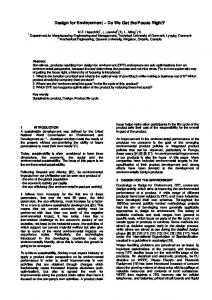
Figure 4. Parts and their mates specification before (a) and after (b) adjustment according to the mates.
Modelica takes information about the mates and produces a corresponding set of Modelica class instances with connections between them. The mass and inertia tensors for each part are computed by SolidWorks. These are extracted and used in Modelica model. Geometry information is saved in a separate STL [17] file for each part. By default the gravity force is applied to the mechanical model. Usually this is not enough for simulation. All external forces that are applied to the bodies, as well as motor forces that are applied to revolute and prismatic joints should be specified. This is done outside the SolidWorks model by adding code for new class instances to the Modelica model. A control subsystem that controls the forces according to a certain plan (mission) can be written in Modelica. If necessary, external code in C can be added to the model. When a Modelica model is simulated, the position, orientation, velocity and acceleration for each part (Body instance) is computed. For Modelica simulation we use the Dymola tool with Modelica support[3].
3.1. Example The example (Figure 4(a)) describes a fragment of the pendulum model. The part P1 has front face (f1) and upper edge (e1). The part P2 has the front face (f2) and bottom edge (e2). There is a mate 1 that specifies that planes of f1 and f2 are coincident. The mate 2 specifies that the edges e1 and e2 are coincident. The SolidWorks system analyzes the mates and adjusts positions of the parts (Figure 4(b)). The system automatically rejects invalid mate combinations. Our translator [7] finds that there is a joint with one rotational degree of freedom between the parts P1 and P2, and calculates the position and orientation of the rotation axis. This pair of mates corresponds to an instance of class RevoluteS from Modelica MBS library with attached Body instance.
M
M
SolidWorks model
Geometry
Mass & inertia
Mates
Translator STL format
Mechanical Modelica model
Optimizer
3.2. Modelica Model Each SolidWorks assembly consists of a set of parts, and it stores a set of mates. All these are validated and translated to a set of Modelica MBS class instances and appropriate connections between them. Mass, position of center of mass and inertia tensor are extracted from the corresponding part documents by SolidWorks. The result of a Modelica model simulation is position, rotation, velocity, acceleration and other physical properties of each Body as functions of time during the simulated time period.
Assembly
Part
Binary form
Non-mechanical model components
Script 3D-Visualizer
Display
Libraries
Modelica execution
Simulation results posiother tions
2D - Graph viewer
4. Translation and simulation Figure 5 represents components of the environment needed for visualization. Our translator from SolidWorks to
Figure 5. The path from SolidWorks model to dynamic system visualization.
5. Visualization The integrated environment includes a visualizer that provides online dynamic display of the assembly (during simulation) or offline (based on saved state information for each time step). The STL format[17] is a very simple format suitable for visualization. All surfaces are divided into triangles and the the coordinates of the triangle vertices, as well as normal vectors of the triangles, are listed in the STL-file. The visualizer loads the corresponding STL file for each part and optimizes it for rendering. After that, rendering is performed by OpenGL [8] library functions. During optimization the vertices positioned very close are merged together. Optimized STL code is stored in a binary file for future use. The user of the visualizer can alternatively utilize the pop-up menu system, keyboard shortcuts, or a command string in order to control various options. We found that the following options (that can be turned on and off) should be available, and we have implemented them. — Rotating the camera in 2 degrees of freedom (DOF), moving the camera in 3 DOF, zooming in and out. — Using perspective and orthographic projection. — Display of a part as a wire-frame, filled with certain color, using a lighting model with certain light sources, or hiding a certain part. — Display of an application-specific landscape, for instance, road for car simulation, or a runway surrounded by hilly landscape for flight simulation. Such a landscape can be created as a SolidWorks assembly that does not move, or directly in C using OpenGL. — Display of planned trajectory (mission) of some parts. — Display of actual trajectory of some parts. — Display of origin and coordinate axes (local for bodies and global one) as well as grid lines. — Display pseudo-shadow. The pseudo-shadow is not depending of light at all. We found that for flight simulation it is convenient to display a projection of vehicle and trajectory on the ground plane. — Synchronization of animation with machine clock. — Starting, stopping, continuing animation, stepping forward and backward. — Targeting camera center of view on a particular part, so that camera follows the part all the time. — Rotating camera together with the target part. The integrated system has been used for modeling industry robot behavior as well as helicopter flight simulation (Figure 6). We have designed a robot and helicopter control models and performed design optimization for the control system [18, 15]. The helicopter is designed in SolidWorks and consists of 10 parts, 4 revolute and 2 prismatic joints.
Figure 6. Helicopter dynamic visualization. It is possible to export the visualization to the 3D Studio MAX [1] (to create and save movies) and MultiGen[12] on SGI (to design Virtual Reality applications).
6. Related Work Our approach has similarities to the Working Model 3D tool [19]. This tool permits construction of a mechanical model with joints (free and motor-controlled), springs, dampers and ropes. It also has built-in collision detection options. Working Model 3D can import assemblies from SolidWorks. However Working Model 3D is a closed system and userdefined control code can be used there in a very limited way. On the contrary in Modelica we specify arbitrary control algorithms for mechanical and mechatronic models. Working Model 3D is limited to certain types of mechanical systems, whereas Modelica supports general multi-domain modeling. Similar mechanical simulation features are available in some other advanced CAD tools.
7. Future work 7.1. Using STEP/EXPRESS for Contact Computation STEP (Standard for the Exchange of Product data)[6, 14] is an international standard for data exchange. It includes a language called EXPRESS, that can be used for exchanging advanced geometric information between CAD/CAM systems. This is an advanced file format where the geometry of the solids is represented in a more mathematical way than in STL. This format could be useful when calculating points
of contact between parts or if a representation of the part geometry on closed form was to be included in the Modelica model.
7.2. True Multidomain Applications Modelica is suitable for multiple application domains. Components from several domains (mechanical, electrical, hydraulic simulation) can be used within the same Modelica model. For instance, electrical components can be combined with mechanical components in the model. The electrical parts can be written by hand, or designed using a block-oriented editor, or extracted from an electric CAD system. The generated Modelica code for electrical components in combination with a mechanical design tool produces a multidomain Modelica model.
8. Conclusions An integrated environment for simulation of multidomain models has been implemented using Modelica as a standard model representation. The user can work with arbitrary SolidWorks models, extend the corresponding Modelica model in various ways, and analyze the simulation results in high performance visualization environment. A complex model such as a pendulum consisting of seven bars can be created in ten minutes. It is simulated 5-7 times faster than corresponding model in Working Model 3D [19]. The helicopter and industrial robot models [18, 15] were successfully designed and simulated.
[6] ISO 10303, Industrial Automation Systems and Integration - Product Data Representation and Exchange, ISO TC 184/SC4, 1992. [7] H. Larson, Translation of 3D CAD models to Modelica, Master Thesis, IDA, Link¨oping Univ., Sweden, April 1999. [8] J. Leech, OpenGL http://reality.sgi.com/opengl
Web
Site,
[9] S.E. Mattsson, H. Elmqvist, M. Otter, Physical system modeling with Modelica, Control Engineering Practice, 1998, vol. 6, pp. 501–510. [10] Modelica WWW site, http://www.modelica.org
Modelica
[11] Modelica activities in PELAB Group, Link¨oping http://www.ida.liu.se/˜pelab/modelica
Group, PELAB, University,
[12] Multigen, OpenFlight section, MultiGen-Paradigm, Inc., http://www.multigen.com [13] M. Otter, Objektorientierte Modellierung mechatronischer Systeme am Beispiel geregelter Roboter. Dissertation, Fortschrittberichte VDI, Reihe 20, Nr. 147, 1995. [14] J. Owen, STEP – An Introduction, Information Geometers Ltd., 1993, ISBN 1-874728-04-6.
9. Acknowledgments The Modelica definition has been developed by the Eurosim Modelica technical committee [10] under the leadership of Hilding Elmqvist (Dynasim AB, Lund, Sweden). The work has been supported by the Wallenberg foundation as part of the WITAS project [18].
[15] J. Parmar, Modeling Autonomous Helicopters using Modelica, Master Thesis, IDA, Link¨oping Univ., Sweden, To appear in June 1999. [16] SolidWorks, SolidWorks http://www.solidworks.com
Corporation,
[17] StereoLithography Interface Specification, 3D Systems, Inc., Valencia, CA 91355. Available via http://www.vr.clemson.edu/credo/rp.html.
References [1] 3D Studio Max, Autodesk Inc., http://www.ktx.com [2] Cult 3D Home Page, Cycore AB, http://www.cykar.se [3] Dymola Home Page, http://www.dynasim.se
[5] P. Fritzson, V. Engelson, Modelica – A Unified ObjectOriented Language for System Modeling and Simulation, In Proc. of Eur. Conf. on Object-Oriented Progr. (ECOOP98), Brussels, July 20–24, 1998.
Dynasim
AB,
[4] H. Elmqvist, S. E. Mattsson. Modelica – The Next Generation Modeling Language – An International Design Effort. In Proceedings of First World Congress of System Simulation, Singapore, September 1–3 1997.
[18] WITAS group, The Wallenberg Laboratory for Research on Information Technology and Autonomous Systems, Link¨oping University, http://www.ida.liu.se/ext/witas [19] Working Model , http://www.krev.com
MSC.Working
Knowledge,