A Destination Prediction Method Using Driving Contexts and Trajectory for Car Navigation Systems Kohei Tanaka†
Yasue Kishino‡
Tsutomu Terada∗
Shojiro Nishio†
† Grad. of Information Science and Technology, Osaka University ‡ NTT Communication Science Laboratories ∗ Grad. of Engineering, Kobe University
† {tanaka.kohei,
nishio}@ist.osaka-u.ac.jp, ‡
[email protected], ∗
[email protected]
ABSTRACT Car navigation systems provide the best route to a destination quickly and effectively. However, during daily driving, this information is not necessary since drivers already know the route to the destination very well. In addition, it is time-consuming for drivers to input the destination. Thus, our research group has proposed a new car navigation system that provides information related to the destination by predicting the user’s destination automatically. We propose the use of a new method that predicts the destination on the basis of the driving trajectory and the contexts in which the user drives. A system that uses our method knows the destination without user interaction and provides information related to the correct destination.
Categories and Subject Descriptors H.4.0 [Information Systems Applications]: General; I.5.5 [Pattern Recognition]: Design Methodology—Classifier design and evaluation; D.2.10 [Software Engineering]: Design—Methodologies
2. DESTINATION PREDICTION FOR CAR NAVIGATION SYSTEM
General Terms Algorithms
Our system[4] has a structure as shown in Figure 1. Because of space limitations, we have omitted the details and simply show the key features. This system is implemented on a PC-based system and a commercial car navigation system using Java.
Keywords Car navigation system, Destination prediction
1.
These mechanisms are used only in the navigated situation where the user does not know the route to the destination and the system navigates the user to the destination. However, in daily driving i.e., to work or for shopping we are mostly in a non-navigated situation where we are very familiar with the route to the destination. Most these functionalities are not used in everyday driving. Therefore, our research group has developed a new navigation system that predicts the driver’s purpose and destination, and automatically presents information that is valuable even in a non-navigated situation. For example, when the system predicts the destination as Train Station ’X’, it presents the train schedule at the estimated arrival time and the traffic information on the predicted route. The method of predicting the destination that we previously developed had some problems because only the driving trajectory was used. We have investigated the reasons for errors in the previous method, and we propose the use of a new way to predict the destination. This method changes dynamically on the basis of the type of road driven on.
INTRODUCTION
2.1 Service Scenario
Recently, the car navigation system has become more and more popular all over the world. It consists of various functions, such as vehicle positioning, route retrieval for the destination, map database management, and visualization. Many researchers and companies have developed mechanisms for these functions and applied them to navigation systems.
The following are some examples of how our system presents the information related to the destination and the route: • The system automatically predicts that the user destination is a shopping mall and presents information about another parking lot because the route to the primary lot is now congested. • The system automatically predicts that the driver is taking their passenger to the station and presents a train schedule with the estimated arrival time.
Permission to make digital or hard copies of all or part of this work for personal or classroom use is granted without fee provided that copies are not made or distributed for profit or commercial advantage and that copies bear this notice and the full citation on the first page. To copy otherwise, to republish, to post on servers or to redistribute to lists, requires prior specific permission and/or a fee. SAC’09 March 8-12, 2009, Honolulu, Hawaii, U.S.A. Copyright 2009 ACM 978-1-60558-166-8/09/03 ...$5.00.
• The system recognizes that the destination is a restaurant and recommends several menu items. We assume that the system presents various pieces of information at the same time, which are related to destinations
190
Sensor Data from the Car (GPS, Veracity,etc)
Dest. A
road link
d c Destination Prediction
road link
Dest. B e
Purpose Prediction
Trajectory DB
Frequency
a Destination
Information Retrieval
Purpose
Information Presented
Information Display
b
Information Retrieval
a b c d e
Destination A B 10 10 0 10 0
2 1 1 0 2
Figure 2: Various of road link
Navigation Information DB
100 90 80 70 60
“Shin-Osaka ḛSin-Osaka StationḜ Station”
% 50
Bound for Osakaᾉ 9:30, :47 Bound for Tokyoᾉ 9:32, :45
40 30 20
ḛGet homeḜ ?
10
You should go to gas station. Fuel Empty!!
0 2000
4000
6000
8000
10000
12000
distance from departure (m) Destination A
Destination B
Destination C
Figure 1: Structure and snapshot of our system
Figure 3: Result of prediction using BM
with higher probability. This is because, while the system does not always predict destinations correctly, its purpose is to present correct information for as long as possible. As shown in Figure 1, since the system also needs to display the map and the current location of the vehicle, it presents 4 pieces of information at most.
destination A is quite higher and the system presents the correct information related to A. On the other hand, when the user is driving around 3000m from the departure, the probability of destination A is lower than the others and the system cannot present the correct information.
2.2 Conventional prediction of destinations
3. PROPOSED METHOD
Our research group has proposed the use of a simple destination prediction method, Basic Method (BM) which calculates the degree of concordance between the route from the departure and stored trajectories. It, as shown in Figure 2, uses a data model that manages routes as a set of directed road links and the system records the transition history of road links. The system predicts destinations by using the following formula (1).
We need a way of predicting destination that predicts the correct destination with a higher probability. To do this, we investigated the characteristics of changing the prediction probability through pilot studies, and proposed a new destination prediction method that varies dynamically with the situation. First, we extracted driving road links that have effect on predictions. From the results of our previous investigation, we confirmed that the prediction result often worsened when we drove along alternative ways or along arterial ways that were frequently used in other drives. In the following sections, we discuss this in detail.
Pij = (1 − α)
Nij + αP(i−1)j Ni
(1)
The probability that user at link i goes to destination j is given by Pij . The past frequency of the visiting road link i is given by Ni , and Nij means the frequency of going to destination j by i. The coefficient to control the weight of considering past routes for calculating Pij is given by alpha, and it is set from 0 to 1. The system recalculates the probabilities for all destinations when the user transits to another road link. Note that P0j is the rate of the drives where the destination is j in past drives. We show an example of calculating Pij in Figure 2. When a user drives along link a, PaA and PaB are 83%(= 10/12) and 17%(= 2/12). Next, when he/she arrives at link b, PbA and PbB become 87.1%(= 0.5 × 10/11 + 83% × 0.5) and 12.9%. An example of a prediction result using this method is shown in Figure 3. The figure shows the transition of probability for each destination where the correct destination is A. On the right side of the graph, that is near the destination, the probability of the intended destination being
3.1 Using alternative routes 3.1.1 Problems and issues When we use an alternative way, it has deleterious effect on the accuracy of the prediction. An example is shown in Figure 4; when a user drives along link c instead of one that which he/she usually uses, b, the destination prediction highly depends on the record of c and the probability for the correct destination decreases significantly. After that, when he/she arrives at link d, in most cases, the probability is restored. Thus, the probability temporarily decreases. In this example, when the transition between link a and c occurs, the probability that he/she goes to destination A changes from 83 to 42% while the probability for B rises to 58% from 17%. Next, when he/she arrives at link d, the probability of A is restored to 71%. Since it causes a lack of reliability, incorrect information may thus be presented. As drivers often take a more indirect route for reasons based
191
Dest. A
usual route
AM
d c (alternative way)
BM
Dest. B e
80 90 50 60 70 20 40 0 10 30 (%) Percentage of distance for which the prediction includes the correct destination
Frequency
road link b c d
a b Departure
Figure 5: Evaluation result for method using alternative way
A B 10 1 0 1 10 0
Table 1: Probability of changes in rank for correct destination
Figure 4: Example of using alternative way
Rank up down
on their experience, such as to avoid a red traffic signal or a traffic jam, the system may present information on an undesired destination.
3.1.2 Prediction method considering alternative routes We propose the use of the Alternative way Method (AM) that is suited for use on alternative routes to resolve the problem described. The main idea is that it changes the weight of past prediction probability on the basis of the situation. Though the weight “α” in Equation (1) is constant in the BM, we change the weight α dynamically to eliminate the loss of predictive accuracy of using the alternative way. In the new method, α and Pij are defined by following equations, respectively. α
=
Pij
=
Ni−1 Ni−1 + Ni Nij Ni−1 + P(i−1)j Ni−1 + Ni Ni−1 + Ni
BM 58.6% (65/111) 41.4% (46/111)
AM 61.1% (66/108) 38.9% (42/108)
drives along link b, as shown in Figure 6, the probability of Destination A decreases significantly since he/she has often used the link b to go to B. When a user drives along link a, the probability of A is 83%. Next, when he/she arrives at link b, this probability decreases to 46%. As a result, the information presented about destination A disappears during the drive on link b.
3.2.2 Prediction method with arterial way By using the data for each departure, we may be able to predict the correct destination. We call this method the Departure Method (DM). An example is shown in Figure 6. The system predicts the correct destination, A, with 83% probability by using the refined data while the prediction rate gained in the BM is 46%.
(2) (3)
3.2.3 Evaluation
As shown in the equation (2), Ni means the frequency of the visiting road link i in the past. By using this equation, the frequency of using the road is considered as the significant factor.
We evaluated the DM by comparing it with the BM using the same data as that used in the evaluation in the last section, which is the trajectory data of 104 drives. To find the difference between both methods, we compared the number times the prediction probability changed. The evaluation result is shown in Table 2. The probability of the correct destination calculated by the BM decreased more frequently than that calculated by DM. Therefore, the DM predicts the correct destination for a longer time than the BM does. One of the reasons is that the passed route becomes a tree-shaped structure using the DM and it can be used to factor in the user’s behavioral characteristics, such as he/she often drops in somewhere on the way home from school. On the other hand, it is difficult to use the DM to collect data on driving. The data gained from the DM in Table 2 are fewer than those gained from the BM. This fact brings new problems that the DM cannot predict the correct destination where a user has visited it many times from other places but he/she has not been there from the present departure point. Moreover, the prediction result is easier to change since the DM has fewer training data than the BM does. Thus, both methods have merits and demerits.
3.1.3 Evaluation We evaluated the AM by comparing the ratio that the prediction results include the correct destination in the Top1 or Top-4 accurately predicted distances. In the evaluation, we use the trajectory data of 104 drives by two test subjects during 4 months. The result is shown in Figure 5. The ratio of Top-1 improves about 2% while, compared with BM, the ratio of Top-4 does not change. In addition, we evaluated the total count of changes in rank for the correct destination. The result is shown in Table 1. Using AM decreases that the rank for the correct destination decreases. These results mean that the AM is more suitable for predicting destination but the difference in accuracy is not significant.
3.2 Using arterial way 3.2.1 Problems and issues
3.3 Context based prediction
When we use an arterial way that is used a number of times, such as one used on a commute, the prediction probability highly depends on ity and the system cannot predict a less commonly used destination. For example, when a user
Though the BM, the AM, and the DM predict the destination using only the driving trajectory, predicting destinations where they are in the same direction or they are
192
Table 3: Number of visits for each context Context (time of day, day of week, weather, number of passengers, weight of baggage) (morning, holiday,sunny, single, light) (morning, holiday,sunny,single, heavy) : (night, workday, rainy, multiple, heavy)
day of week
Table 2: Probability of increase/decrease for correct destination
Increase Decrease
BM 65.0%(316/486) 35.0%(170/486)
d
Dest. B a b (arterial way)
Departure C
weather
weight of baggage
time of day
DM 80.7% (167/207) 19.3% (40/207)
Dest. A
Destination A B … Z 1 2 … 1 1 4 … 1 … 1 3 … 5
number of passengers
destination
passing Area 1
Total frequency road link A B a 10 2 b 10 100 d 10 0
passing Area i
Figure 7: Our structured Bayesian network Table 4: Particle size of each context Context Particle size time of day morning,noon,night weekday,holiday day of week weather sunny,rainy number of passengers single,double,multiple weight of baggage light,heavy
Frequency from C road link A B a 10 2 b 10 2 d 10 0
Figure 6: Use of an arterial way located close to each other is difficult. Therefore, we propose the use of the Context Method (CM) that predicts the destination using driving context such as the time of day, the day of the week, the number of passengers, and the weather. In addition, since the transition sequence of the vehicle’s approximate positions also explains the context of driving, we use area transitions by dividing the field into two-dimension lattices. We made the CM by using a Bayesian network, which is often used to predict user behaviors on the basis of his/her past behaviors. In our method, we structured the network as shown in Figure 7. This network predicts the destination by using a table that stores the number of visits for every driving context. An example is shown in Table 3, and Table 4 shows the granularity of each context. We supposed that the context can be recognized automatically and confirmed that most contexts can be recognized using by a set of sensors .
The type of road classified by the change of probability and how often they are used to get to a given destination are shown in Table 5. The probability changes are different for each destination. Therefore, even the same road can be classified as a different type.
3.4.1 Detecting the type of road
First, we used the data from the previous sections to investigate how frequent the change in probability occurs. The result is shown in Table 6. Even for the correct destination, the correctly predicted rate when the prediction probability in both methods increases is only 61.9%. Therefore, it does not necessarily mean that it a predicted destination is the correct one when the probability of both methods increases. On the other hand, when both probabilities decrease, the rate that the destination is correct is 1.2%. Thus, when the probabilities of both methods decrease for a destination, it 3.4 Prediction destination by using Hybrid method is not the correct one and the present road is not used to go to that place. The case where the results from the two methWe proposed several destination prediction methods in ods are different rarely occurred; the rate is approximately previous sections. However, they have both merits and de4%. From the table, the probability increasing in the DM merits in different situations. Therefore, we propose the use for the correct destination happens more frequently than of Hybrid Method (HM) that changes prediction method dythat in the AM does in such a situation. Therefore, when namically with the type of road driven on. There are several the result of both methods is different, the DM predicts the methods finding what road is being used. One of them is destination more accurately than the AM does. by using a map database. Though it is simple, the road These results suggest that when both probabilities inis different on every drive and the prediction method may crease, the prediction method needs to keep the probabilnot work well. Thus, we consider that the road type can be ity. This suggests that the predicted destination is likely classified by the characteristics of the changes in probabilto be the correct destination. On the other hand, when ity for each prediction method. We used the changes of the both probabilities decrease, the prediction method needs to prediction result gained from the AM and the DM since the decline the destination since the probability that it is the CM result is almost constant.
193
Type of road i ii iii iv
Table 5: Type of the AM DM Increase Increase Increase Decrease Decrease Incresase Decrease Decrease
road according to the change of probability Meaning of the road often used for the destination often used from other departures for the destination often used for the destination though often used for other places rare used for the destination
Table 6: Number of probability changes Type All destinations Correct destination (Occurrence rate) (Correctly predict rate) i 239 times 148 times (12.6%) (61.9%) ii 38 times 11 times (2.0%) (28.9%) iii 33 times 19 times (1.7%) (57.6%) iv 1586 times 19 times (83.6%) (1.2%)
CM DM Top1 Top4
AM 㻜0
20 㻜㻚㻞
40 㻜㻚㻠
60 㻜㻚㻢
80 㻜㻚㻤
100㻝 (%)
Percentage of distance for which the prediction includes correct destination
Figure 8: Pprediction results in type (i)
CM DM Top1 Top4
AM
correct one decreases. When the change in both probabilities is different, the implications for the prediction method are not yet clear. We now discuss the road types as well as the implications of our experiments for which method is better for prediction.
㻜0
20 㻜㻚㻞
40 㻜㻚㻠
60 㻜㻚㻢
80 㻜㻚㻤
100㻝 (%)
Percentage of distance for that the prediction includes correct destination
Figure 9: Prediction results in type (ii)
CM
3.4.2 Conducting the hybrid method Using HM changes the prediction methods dynamically with the road types. Using the same data as those in the pilot study, we applied the prediction methods (AM, DM, and CM) to the each road type. We tried all combinations between the types of road and the methods and found the best combination of the prediction methods. We evaluated them by the ratio that the prediction results include the correct destination in the Top-1 or Top-4 in all the distances driven. The reason is that our navigation system presents some pieces of information about the topside of the prediction results. What is important is not that the correct destination joins the Top-1, but it can be in the top group. The results are shown in Figure 8 - 11. In the evaluation, we tried all combinations of prediction method and calculated the probabilities. Each figure shows that the average ratio of the driving distance focused on one type of the road. The correct destination is Top-1 or Top-4 when the probabilities of the both methods are increasing, i.e., type (i), is shown in Figure 8. In the same way, Figure 9 shows the results of type (ii), in which the probability of AM increases and the probability of DM decreases. The results of type (iii), in which the AM decreases and the DM increases are shown in Figure 10. The results of type (iv), in which the results of the both methods decrease are shown in Figure 11. From the results, all the prediction methods except CM predict the correct destination move accurately in the type (i) and (iv). In type (ii), there is not much difference of each method. In type (iii), the DM is better adapted to predict for Top-1 and the AM is better for Top-4. Moreover, the DM is the best in type (i), AM is the best in type (iv), and in type (ii) the CM is the best for Top-4 and AM is the best for Top-1 though these results do not show significant
DM Top1 Top4
AM 㻜0
20 㻜㻚㻞
40 㻜㻚㻠
60 㻜㻚㻢
80 㻜㻚㻤
100㻝 (%)
Percentage of distance for that the prediction includes correct destination
Figure 10: Prediction result in type (iii)
CM DM Top1 Top4
AM 㻜0
20 㻜㻚㻞
40 㻜㻚㻠
60 㻜㻚㻢
80 㻜㻚㻤
100㻝 (%)
Percentage of distance for that the prediction includes correct destination
Figure 11: Prediction result in type (iv)
differences. From these results, we propose the use of HM classified by the Table 7 for Top-4 prediction. Additionally, since predicting the Top-1 group is also important in areas such as using voice guides, we propose the use of HM with the classification shown in Figure 8 for the Top1 prediction.
3.4.3 Evaluation We have implemented HM on the prototype system. We evaluated the method using half of the data for training and the other data for evaluation. The data is the trajectory for a 4-month period of a single person driving by a person. In other words, we evaluated the effectiveness of our proposed method in the case where the user has used our system for
194
Table 7: Hybrid Type AM i Increase ii Increase iii Decrease iv Decrease
method for Top-4 prediction DM Prediction method Increase DM Decrease CM Decrease AM Decrease AM
HM for Top-1 HM for Top-4 AM DM CM
Table 8: Hybrid method for Top-1 prediction Type AM DM Prediction method i Increase Increase DM ii Increase Decrease AM Decrease Increase DM iii iv Decrease Decrease AM
Top1 Top4
BM 0
20
40
60
80
100 (%)
Percentage of distance for which the prediction includes correct destination
Figure 12: Performance of proposed method in the early stages.
5. CONCLUSION
a training term of two months. The results are shown in Figure 12. It shows how long the information related to the correct destination is presented. We found that both of our methods can predict the correct destination with a rate of accuracy approximately 20% higher than other methods in Top-1 and 10% higher than those used in Top-4. The reasons why the DM is worse than BM may be that 2 months is not enough collect all the training data needed to to predict the correct destination.
4.
We have proposed the use of a new destination prediction method that factors in the driving trajectory and common contexts of daily driving that would be useful to include in a car navigation system. We evaluated the proposed method on the basis of a prototype system. We clarified the situations in which our proposed method works well, and we propose integrating these proposed methods in different ways on the basis of the changes in the situation. Our future work is to bring out the relation between the amount of training and suitable prediction methods, and we will carry out experiments with more users to evaluate the proposed method.
RELATED WORK
There are several pieces of research on destination prediction based on driving trajectory. For example, one method is to divide a map into grids by latitude and longitude and transform the driving route to the grids [1]. The current passed grids are compared with the previous passed grid and the concordance is measured. It also supposes that the current position is important and gives a large weight to the current grid like the BM does. Since this method is similar to the BM, it has also the problems when the driver chooses driving alternative and arterial routes. One method is to use the difficulty of estimating the arrival place as a cross-point as a node of the network and show the difficulty of predicting the destination by using node transitions [5]. Thus, it predicts the destination and it also defines the entropy as the characteristic of difficulty that was calculated by driving times. Using the entropy, we can know the degree of certainty of the prediction. There is work on a method that is used to learn and infer the user’s daily movements using a hierarchical Markov model [2]. This model uses the GPS data logs to accurately predict the goals of a person and recognizes the situations in which the user performs unknown activities. However, their experiments are executed in a specific situation in which the user’s movement is only between 5 points. Neither method can adapt to more complex situations such as driving alternative and arterial ways. There are also many studies that predict user behaviors using his/her locations. One of them describes a way to predict the change of transportation mode using Bayesian networks [3]. Their network is complex and constructed on the basis of general knowledge. If we structure our CM, in this way, the predictive accuracy may not be much higher
6. ACKNOWLEDGMENTS This research was supported in part by a Grant-in-Aid for Scientific Research (A)(20240009), Priority Areas (19024046), and JSPS Fellows (1955371) of the Japanese Ministry of Education, Culture, Sports, Science and Technology, and by the Global COE program “Center of Excellence for Founding Ambient Information Society Infrastructure.”
7. REFERENCES [1] M. Kobayashi et al. The arrival place presumption mechanism applied to an information filtering system for in-vehicle navigation systems. Transactions of Information Processing Society of Japan, 45(12):2688–2695, 2004. [2] L. Liao et al. Learning and inferring transportation routines. Artif. Intell., 171(5-6):311–331, 2007. [3] D. J. Patterson et al. Inferring high-level behavior from low- level sensors. In Proc. of The Fifth International Conference on Ubiquitous Computing (UbiComp2003), pages 73–89, 2003. [4] T. Terada et al. Design of a car navigation system that predicts user destination. In Proc. of Int’l Workshop on Tools and Applications for Mobile Contents (TAMC), pages 54–49, 2006. [5] M. Yoshioka and J. Ozawa. Destination entropy for arrival place presumption from car driving route history. Transactions of Information Processing Society of Japan, 46(12):2973–2982, 2005.
195