Int. J. Procurement Management, Vol. 3, No. 3, 2010
A deterministic order level inventory model for deteriorating items with two storage facilities under FIFO dispatching policy Chandra K. Jaggi* and Priyanka Verma Department of Operational Research, Faculty of Mathematical Sciences, New Academic Block, University of Delhi, Delhi-110007, India Fax: 91-11-27666672 E-mail:
[email protected] E-mail:
[email protected] E-mail:
[email protected] *Corresponding author Abstract: Generally, two warehousing inventory models adopt the last-in-first-out (LIFO) dispatch policy. According to this policy, the items that are stored last are used first. This approach might not appear appropriate in case of deteriorating goods. First-in-first-out (FIFO) dispatch policy aids in preserving the freshness of commodities that tend to deteriorate and is therefore, widely preferred for facilities that store them. Adoption of the FIFO policy yields fresh and good conditioned stock thereby resulting in customer satisfaction. Organisations that deal in perishable goods survive and thrive on this principle. In this paper, Sarma’s (1987) LIFO model for ‘deteriorating items with two storage facilities’ has been revisited under FIFO dispatch policy. The two models have been compared using various parameters like holding costs and deterioration rates in both the warehouses and appropriate dispatch policy has been suggested. The results have been validated with the help of a numerical example. Sensitivity analysis has also been performed to study the impact of various parameters on the optimal solution. Keywords: inventory; warehouse; deterioration; shortages; first-in-first-out; FIFO; last-in-first-out; LIFO. Reference to this paper should be made as follows: Jaggi, C.K. and Verma, P. (2010) ‘A deterministic order level inventory model for deteriorating items with two storage facilities under FIFO dispatching policy’, Int. J. Procurement Management, Vol. 3, No. 3, pp.265–278. Biographical notes: Chandra K. Jaggi is an Associate Professor in the Department of Operational Research, University of Delhi, India. He earned his PhD and MPhil in Inventory Management and Masters in Operational Research from Department of Operational Research, University of Delhi. His teaching includes Inventory Modelling and Financial Management. His areas of research are production/inventory and supply chain management. He has publications in International Journal of Production Economics, Journal of Operational Research Society, European Journal of Operational Research, International Journal of Systems Sciences, International Journal of Procurement Management, TOP, International Journal of Applied Decision Sciences OPSEARCH, Investigacion Operacional Journal, International Journal of Operational Research, Advanced Modelling and Optimization, etc.
Copyright © 2010 Inderscience Enterprises Ltd.
265
266
C.K. Jaggi and P. Verma Priyanka Verma is a Research Scholar in the Department of Operational Research, Faculty of Mathematical Sciences, and University of Delhi, India. She has completed her MSc in Applied Operational Research in 2003, from University of Delhi. At present, she is pursuing her PhD in Operational Research. Her area of interest is inventory management. She has three research papers published in TOP (Spain), International Journal of Mathematics and Mathematical Sciences (IJMMS) and International Journal of Operational Research (IJOR) and one research paper has been accepted in International Journal of Operational Research (IJOR).
1
Introduction
Usually the two warehousing systems assume that the holding cost of items is more in RW than the owned warehouse (OW) due to additional and modern preserving facilities resulting in lower deterioration rate. To reduce the inventory costs, it would be economical to consume the goods of RW at the earliest. Consequently, the firm stores goods in OW before RW, but clears the stocks in rented warehouse (RW) before OW. This approach is termed as last-in-first-out (LIFO) approach. Another commonly adopted approach called first-in-first-out (FIFO) is more practical. According to this approach, the deteriorating items stored in OW are used prior to the items stored in RW to preserve their freshness and reduce the deterioration rate. This approach is based on the assumption that the RW offers better preserving facilities at lesser holding cost than the OW due an increased competition in warehouse market. In this paper, Sarma’s (1987) model for deteriorating items with two storage facilities under LIFO approach is being revisited and the existing model has been investigated under the FIFO dispatch policy. Further, it is assumed that the holding cost in RW is not necessarily higher in OW. The optimal order size for the period has been obtained and the proposed model is also illustrated with different values of holding costs and different deterioration rates. Sensitivity analysis on various parameters is performed to examine the impact on policy choice.
2
Literature review
The deterioration of inventory in stock during the storage period constitutes an important factor, which has attracted the attention of researchers. Deterioration, in general, maybe considered as the result of various effects on the stock, some of which are damage, spoilage, obsolescence, decay, decreasing usefulness, and many more. The first attempt to obtain optimal replenishment policies for deteriorating items was made by Ghare and Schrader (1963), who derived a revised form of the economic order quantity (EOQ) model assuming exponential decay. These authors studied a model, having a constant rate of deterioration and a constant rate of demand over a finite planning horizon. The model of Ghare and Schrader was extended by Covert and Philip (1973) by introducing variable rate of deterioration. A further generalisation to the above models was proposed by Shah (1977) by considering a model allowing complete backlogging of the unsatisfied demand.
A deterministic order level inventory model for deteriorating items
267
Thereafter, a great deal of research efforts has been devoted to inventory models of deteriorating items. Some of the researchers who extensively examined these models are Montgomery et al. (1973), Rosenberg (1979), Raafat et al. (1991), Wee (1995), Abad (1996), Chang and Dye (1999), Goyal and Giri (2001), Yang (2006), Jaggi et al. (2006), Rong et al. (2008) and others. The general assumption in classical inventory models is that the organisation owns a single warehouse without capacity limitation. But, in practice, when a large stock is to be held, due to the limited capacity of the owned warehouse (denoted by OW), one additional warehouse is required. This additional warehouse may be a rented warehouse (denoted by RW), which is assumed to be available with abundant capacity. A model considering the effect of two-warehouse was considered by Hartley (1976) in which he assumed that the holding cost in RW is greater than that in own warehouse (OW), therefore, items in RW are first transferred to OW to meet the demand until the stock level in RW drops to zero and then items in OW are released. Sarma (1987) extended Hartley’s model to cover the transportation cost from RW to OW that is considered to be a fixed constant independent of the quantity being transported. But he did not consider shortages in his model. Goswami and Chaudhuri (1992) further developed the model with or without shortages by assuming that the demand varies over time with linearly increasing trend and that the transportation cost from RW to OW depends on the quantity being transported. In their model, the stock was transferred from RW to OW in an intermittent pattern. However, their work is for non-deteriorating items only. Sarma (1983) developed a two-warehouse model for deteriorating items with the infinite replenishment rate and shortages. Pakkala and Achary (1992) further considered the two-warehouse model for deteriorating items with finite replenishment rate and shortages. Bhunia and Maiti (1998) developed a two-warehouse model for deteriorating items with linearly increasing demand and shortages during the infinite period. Research continues with Zhou (1998), Zhou and Yang (2003), Chung and Huang (2007), Das et al. (2007), Dye et al. (2007), Dey et al. (2008), Hsieh et al. (2008), Niu and Xie (2008) and many more. Moreover, in two warehousing models it is generally assumed that the holding cost of items is more in RW than the OW due to additional cost of maintenance, material handling etc. For example, the RW like ‘central warehousing facility’ generally provides better preserving facility than the OW resulting in a lower deterioration rate for the goods. To reduce the inventory costs, it will be economical to consume the goods of RW at the earliest. Consequently, the firm stores goods in OW before RW, but clears the stocks in RW before OW. But as the competition increases in the warehouse facilities in real world, RW with better preserving facilities, well equipped set ups and other latest facilities are available at lower costs than OW. So the costs can be reduced by using FIFO approach. According to this approach, the perishable and deteriorating items stored in OW are used before the items stored in RW to preserve their freshness and reduce the deterioration rate. In this paper, Sarma’s (1987) LIFO model for deteriorating items with two storage facilities is being revisited under FIFO dispatch policy. Comparison study of two models has also been performed. Results have been validated with the help of a numerical example. Sensitivity analysis has also been performed.
268
3
C.K. Jaggi and P. Verma
Assumptions and notations
The following assumptions are used in developing the model: 1
demand is deterministic and occurs uniformly over the period
2
replenishment is instantaneous
3
the time horizon of the inventory system is infinite
4
lead-time is negligible
5
the OW has a fixed capacity of W units; the RW has unlimited capacity
6
the units in RW are stored only when the capacity of OW has been utilised completely and the goods of RW are consumed only after consuming the goods kept in OW
7
shortages are allowed and completely backlogged.
Notations adopted in this paper are as below: R
the demand rate per unit time
W
the storage capacity of OW
QF
the replenishment quantity per replenishment
SF
the initial inventory for the period
tw
the time at which inventory level reaches zero in OW
t1
the time at which inventory level reaches zero in RW
T
the length of the replenishment cycle which is a prescribed constant
C
the purchasing cost per unit item
π
the shortage cost per unit per unit time
H
the holding cost per unit per unit time in OW
F
the holding cost per unit per unit time in RW
α
the rates of deterioration in OW, 0< α W and zero otherwise. The goods of the RW are consumed only after consuming the goods in OW. By time tw inventory level in OW reaches to zero due to the combined effect of demand and deterioration and the inventory level in RW also reduces from Z to Z0 due to effect of deterioration. By time t1 inventory level in RW reaches to zero due to the combined effect of demand and deterioration. Now both the warehouses get emptied and shortages build up until the end of the period T. The quantity to be ordered will be QF =R (T – t1) + SF. The difference between Z and Z0 in the figure is due to deterioration in RW during (0, tw). Figure 1
Graphical representation of two warehouse inventory system
As described above, the inventory level in the OW during the time interval (0, tw) decreases due to the combined effect of demand and deterioration both. The differential equation describing the inventory level in the OW during this interval is dQ0 ( t ) dt
+ α Q0 ( t ) = − R
for 0 ≤ t ≤ t w ,
(1)
and using the initial condition Q0 (0) = W the solution is R⎞ R ⎛ Q0 ( t ) = ⎜W + ⎟ e−αt − α α ⎝ ⎠
for 0 ≤ t ≤ t w
(2)
noting that at t = tw, Q0 (t) = 0 we get tw =
⎛ αW ⎞ log ⎜ 1 + ⎟ α R ⎠ ⎝ 1
(3)
270
C.K. Jaggi and P. Verma
The holding cost of items in OW in the interval (0, tw) is tw
HC ow =
∫ HQ
0
( t )dt (4)
0
⎛ W − Rt w ⎞ =H⎜ ⎟ α ⎝ ⎠
Now, during the interval (0, tw) all the Z units in RW are kept unused but they are subject to deterioration at the rate of β. So the inventory level in RW reduces to Z0 only due to deterioration. The differential equation describing the state of inventory in this interval is given by dQr ( t ) dt
+ β Qr ( t ) = 0
for 0 ≤ t ≤ t w ,
(5)
After using the boundary condition Qr (0) = Z, the solution is Qr ( t ) = Ze−βt ,
0 ≤ t ≤ tw ,
(6)
Now Qr (tw) = Z0, we have Z 0 = Ze −βtw
(7)
The holding cost of items in RW in the interval (0, tw) is tw
∫
(Z − Z ) 0
FQr ( t ) dt = F
(8)
β
0
Again, during (tw, t1), the stock in RW decreases owing to demand as well as deterioration both. The differential equation describing the state of inventory in this interval is given by dQr ( t ) dt
+ β Qr ( t ) = − R,
t w < t < t1
(9)
After using the boundary condition Qr (tw) = Z0, the solution is Qr ( t ) =
−R ⎛ 0 R ⎞ β ( tw −t ) , + ⎜ Z + ⎟e β ⎝ β⎠
t w < t < t1
(10)
Noting that Qr (t1) = 0 and t* = t1 – tw we get
t* =
⎛ β Z0 ⎞ log ⎜⎜ 1 + ⎟ R ⎟⎠ β ⎝ 1
(11)
The holding cost of items in RW in the interval (tw, t1) is t1
∫
tw
FQr ( t ) dt = F
(Z
0
− Rt*
β
)
(12)
A deterministic order level inventory model for deteriorating items
271
So the holding cost of items in the RW is given by HCrw =
(
F Z − Rt*
)
(13)
β
During the shortage interval (t1, T), the demand at any time t is fully back logged. Thus, the shortage level, S(t) in the OW in this interval satisfies the following differential equation: dS( t ) = − R, dt
t1 ≤ t ≤ T
(14)
After using the boundary condition S(t1) = 0, the solution is S ( t ) = R ( t1 − t ) ,
t1 ≤ t ≤ T
(15)
Therefore, the shortage cost in the interval (t1, T) is T
∫
SC = π S ( t ) dt = π R t1
(T − t1 )2
(16)
2
The quantity deteriorated during the period is given by D = ( S F − Rt1 )
(17)
The total average cost function for the system, KF(SF) is thus, given by the following expression: K F ( SF ) =
1 [CD + HCow + HCrw + SC ] T
(18)
After substituting equations (4), (13), (16), (17) into (18) we get the average cost for the system, KF(SF) which is a function of one continuous variable SF, as given below K F ( SF ) =
⎤ 1⎡ F H πR S − W − Rt* + (W − Rt w ) + (T − t1 )2 ⎥ ⎢ C ( S F − Rt1 ) + T⎣ β F α 2 ⎦
(
)
As t1 = tw + t*, after substituting these values we get, KF ( SF ) =
⎡ ⎛ 1 ⎛ αW ⎞ 1 ⎛ β ( SF −W ) e−β tw 1 ⎢ ⎪⎧ C ⎨SF − R ⎜ log ⎜1+ + log ⎜1+ ⎟ ⎜ ⎜α T⎢ ⎪ R ⎠ β R ⎝ ⎝ ⎝ ⎣ ⎩
⎞ ⎞⎪⎫ ⎟ ⎟⎬ + ⎟⎟ ⎠ ⎠⎪⎭
−β t F ⎪⎧ R ⎛ β ( SF −W ) e w ⎞⎪⎫ H ⎧ R ⎛ αW ⎞⎫ ⎟⎬ + ⎨W − log ⎜1+ ⎨SF −W − log ⎜⎜1+ ⎟⎬ + ⎟ β ⎩⎪ β ⎝ α ⎝ R R ⎠⎭ ⎠⎪⎭ α ⎩
⎛ β ( SF −W ) e−β tw ⎞⎫⎪ πR ⎧ 1 ⎛ αW ⎞ 1 log 1 T log − − + ⎜1+ ⎟⎬ ⎨ ⎟ ⎜ ⎜ ⎟ R R ⎠ β 2 ⎩ α ⎝ ⎝ ⎠⎪⎭
(19)
272
C.K. Jaggi and P. Verma
The necessary condition for minimising KF(SF) is
(
)
∂K F ( S F ) = 0 which gives ∂S F
(
)
C β R + β Z 0 − Re − β t w + F R + β Z 0 − Re − β t w − πβ R (T − t1 ) e − β t w = 0
(20)
The above equation can be simplified using the following approximations, assuming their validity, for the relevant expressions. 2
3
1
⎛ αW log ⎜1 + R ⎝
αW ⎞ αW 1 ⎛ α W ⎞ 1 ⎛ α W ⎞ − ⎜ < 1. ⎟= ⎟ + ⎜ ⎟ − − − −− , for 2⎝ R ⎠ 3⎝ R ⎠ R R ⎠
2
⎛ βZ0 ⎞ β Z0 1 ⎛ β Z0 ⎞ 1⎛ βZ0 ⎞ β Z0 log ⎜⎜1 + − ⎜⎜ < 1. ⎟⎟ = ⎟⎟ + ⎜⎜ ⎟⎟ − − − −− , for R ⎠ R 2⎝ R ⎠ 3⎝ R ⎠ R ⎝
3
e − β tw = 1 − β t w +
4
Second and higher order terms of α, β and terms of αβ are negligible as 0 < α