Int. J. Mathematics in Operational Research, Vol. 7, No. 3, 2015
A partial backlogging inventory model for deteriorating items with time-varying demand and holding cost Debashis Dutta* and Pavan Kumar Department of Mathematics, National Institute of Technology, Warangal – 506004, Andhra Pradesh, India Email:
[email protected] Email:
[email protected] *Corresponding author Abstract: In this paper, we propose a partial backlogging inventory model for deteriorating items with time-varying demand and holding cost. Deterioration rate is assumed to be constant. The demand rate varies with time until the shortage occurs; during shortages, demand rate becomes constant. Shortages are allowed and assumed to be partially backlogged. The backlogging rate is variable and is inversely proportional to the length of the waiting time for next replenishment. Taylor series is used for exponential terms approximating up to second degree terms. We solve the proposed model to obtain the optimal value of order quantity and total cost. The purpose of this paper is to minimise the total cost of inventory with optimal order quantity. The convexity of the cost function is shown graphically. Two numerical examples are given in order to show the applicability of the proposed model. Sensitivity analysis is also carried out to identify the most sensitive parameters in the system. Keywords: inventory model; partial backlogging; time dependant demand rate; deteriorating items. Reference to this paper should be made as follows: Dutta, D. and Kumar, P. (2015) ‘A partial backlogging inventory model for deteriorating items with time-varying demand and holding cost’, Int. J. Mathematics in Operational Research, Vol. 7, No. 3, pp.281–296. Biographical notes: Debashis Dutta is currently a Professor in the Department of Mathematics at the National Institute of Technology, Warangal in India. He holds a PhD in Operations Research. He teaches optimisation techniques and statistics. His prime research interest is in the field of mathematical programming, operations research, uncertainty and atmospheric modelling. Pavan Kumar is currently a PhD candidate and SRF-UGC in the Department of Mathematics at the National Institute of Technology, Warangal, India, under the supervision of Prof. D. Dutta. From CCS University, Meerut, India, he received his BSc in Mathematics and MSc in Mathematics. His current research interests include operations research and optimisation techniques.
Copyright © 2015 Inderscience Enterprises Ltd.
281
282
1
D. Dutta and P. Kumar
Introduction
In the literature regarding inventory models, there are four types of demand: constant demand, time-dependent demand, probabilistic demand and stock-dependent demand. But in practical life it is observed that demand of goods does not remain constant. Rather, it varies with time or price or even with the instantaneous level of inventory. Normally, we encounter products such as fruits, milk, drug, vegetables, and photographic films etc. which have a defined period of life time. Such items are referred as deteriorating items. Deterioration means damage, spoilage, dryness, vaporisation, etc. Due to deterioration, inventory system faces the problem of shortages and loss of good will or loss of profit. So, the deterioration must also be considered in inventory control models. In literature, there are so many papers on determination of inventory level of deteriorating items with shortages and without shortage.
2
Literature review
Harris (1915) described the first economic order quantity (EOQ) model for constant and known demand. Then some researchers considered the variable demand such as time dependant and stock dependant. Ghare (1963) proposed a model for exponentially decaying inventory. Later, inventory with deteriorating items were studied by several researchers. Nahmias (1975a, 1975b) proposed a model for optimal ordering for perishable inventory, and then he compared the alternative approximations for ordering perishable inventory. Inventory models with time dependent demand rate were discussed by Sivazlian and Stanfel (1976). Nahmias and Pierskalla (1976) proposed a two-product perishable/non-perishable inventory problem. Dave and Patel (1981) proposed a (T, si)-policy inventory model for deteriorating items with time proportional demand. Chung and Ting (1993) proposed a heuristic for replenishment of deteriorating items with a linear trend in demand. They considered time dependant demand rate. Due to shortages, the backlogging occurs. Sometimes, researchers assumed partial backlogging while some researchers considered fully backlogged. In reality, it is seen that during the shortage period either all customers wait until the arrival of next order (completely backlogged) or all customers leave the system (completely lost). However, it is more reasonable situation to consider that, some customers are able to wait for the next order to satisfy their demands during the stock out period, while others do not wish to or can wait and they have to fill their demands from other sources (partial back order case). The length of waiting time for the replenishment is the main factor for determining whether the backlogging will be accepted or not. For fashionable commodities and high-tech products with short life cycles, the backorder rate is diminishing with the length of waiting time. Customers who experience stock-out will be less likely to buy again from the suppliers, they may turn to another store to purchase the goods. The sales for the product may decline due to the introduction of more competitive product or the change in consumers’ preferences. The longer the waiting time, the lower the backlogging rate is. This leads to a larger fraction of lost sales and a less profit. As a result, taking the factor of partial backlogging into account is necessary.
A partial backlogging inventory model for deteriorating items
283
Abad (1996) studied an inventory model for optimal pricing and lot-sizing under conditions of perishability and partial backordering. Jalan et al. (1996) assumed the deterioration as a two parameter Weibull distribution, and then they proposed an EOQ model for items with Weibull distribution deterioration shortages and trended demand. Chang and Dye (1999) developed an EOQ model for deteriorating items with time varying demand and partial backlogging. Abad (2001) proposed an optimal price and order-size for a reseller under partial backlogging. Goyal and Giri (2001) proposed a model for recent trends in modelling of deteriorating inventory. Ouyang et al. (2005) presented an inventory model for deteriorating items with exponential declining demand and partial backlogging. The rate of deterioration is assumed to be constant and the backlogging rate is inversely proportional to the waiting time for the next replenishment. Dye (2007) developed two inventory models: one on determining optimal selling price and lot size with a varying rate of deterioration and exponential partial backlogging, and other on joint pricing and ordering for a deteriorating inventory with partial backlogging. Teng et al. (2007) studied the comparison between two pricing and lot-sizing models with partial backlogging and deteriorating items. Alamri and Balkhi (2007) proposed a model for the effects of learning and forgetting on the optimal production lot size for deteriorating items with time varying demand and deterioration rates. In real-life inventory model, the holding cost is also time dependant. Roy (2008) considered the time varying holding cost, and then he proposed an inventory model for deteriorating items with price dependent demand and the time varying holding cost. Skouri et al. (2009) proposed some inventory models with ramp type demand rate, partial backlogging and Weibull deterioration rate. Shah and Shukla (2009) developed an inventory model for waiting time partial backlogging and deteriorating items. Nahmias (2009) developed several inventory models with production and operations analysis. Mandal (2010) proposed an EOQ inventory model for Weibull distributed deteriorating items under ramp type demand and shortages. Hung (2011) proposed an inventory model with generalised type demand, deterioration and backorder rates. Sana (2010a) proposed inventory models with time varying deterioration and partial backlogging to determine the optimal selling price and lot size. Further, Sana (2010b) considered a multi-item EOQ model of deteriorating and ameliorating items where demand influenced by enterprises’ initiatives. An EOQ model with price-sensitive demand for perishable items was proposed by Sana (2011). Roy et al. (2011a, 2011b) proposed inventory models for imperfect items in a stock-out situation with partial backlogging. He and Wang (2012) developed a model for the analysis of production-inventory system for deteriorating items with demand disruption. Kumar et al. (2012) proposed some EOQ models with ramp type demand, partial backlogging and time dependent deterioration rate in fuzzy environment. Shah et al. (2012) proposed a model for optimisation inventory and marketing policy for non-instantaneous deteriorating items with generalised type deterioration and holding cost rates. Pal et al. (2013) solved a distribution-free newsvendor problem by considering non-linear holding cost. Fashion and seasonal products are characterised by unpredictable demand. The demand of some items, especially seasonal products like seasonable garments, shoes, etc. is low at the beginning of the season and increases as the season progresses, i.e., it changes with time. Most of these products have a lifespan that ranges between three and six months – a very short window in which to make the right calls on demand and
284
D. Dutta and P. Kumar
procurement and achieve profits. How do managers at firms selling such products plan for a season? How do they decide how much to order, when to schedule shipments and how much to mark down prices to reduce season-ending inventory as much as possible? In this paper, we develop a deteriorating inventory model with time dependent demand rate. The deterioration rate is assumed to be a constant; the unsatisfied demand is partially backlogged. The backlogging rate is variable and is inversely proportional to the length of the waiting time for next replenishment. Our aim is to minimise the total cost of inventory with optimal order quantity and optimal time of inventory exhausting. This paper is organised as follows: Section 2 describes the notations and assumptions, Section 3 presents the mathematical formulation of the problem, Section 4 provides a numerical example to illustrate the proposed inventory model, Section 5 discuses the sensitivity analysis, and finally Section 6 proposes the conclusions.
3
Notations and assumptions
Throughout this paper, the following notations and assumptions are used:
3.1 Notations c1
holding cost per unit per time unit
c2
purchase cost per unit
c3
ordering cost per order
c4
shortage cost per unit per time unit
c5
cost of lost sales per unit
θ
deterioration rate
T
cycle time (decision variable)
t1
time at which shortage starts, i.e., inventory exhausted time, (decision variable), 0 ≤ t1 ≤ T
T – t1
length of waiting time
W
maximum inventory level during a cycle of length T
DB
maximum amount of demand backlogged during a cycle of length T
Q
(= W + DB) order quantity during a cycle of length T
CH
inventory holding cost per cycle
CD
deterioration cost per cycle
CS
shortage cost per cycle
CL
lost sales cost per cycle
A partial backlogging inventory model for deteriorating items C *
285
average total cost per time unit per cycle
X
optimal value of X, where X is any variable
I(t)
inventory level at time, 0 ≤ t ≤ T
I1(t)
inventory level at time t ∈ [0, t1]
I2(t)
inventory level at time t ∈ [t1, T].
3.2 Assumptions 1
⎧ D1 + β t , for 0 ≤ t < t1 , where D1, D2, and β > 0 are arbitrary Demand rate, R (t ) = ⎨ for t1 ≤ t ≤ T ⎩ D2 , constants.
2
Inventory system involves only one item.
3
Planning horizon is infinite.
4
Replenishment rate is assumed to be infinite, which results the Lead time to be zero, i.e., there is no time-lag in delivery of order.
5
Rate of deterioration is constant, θ (0 < θ < 1), and it occurs as soon as items are received into inventory. There is no replacement or repair of deteriorated units.
6
For the time-range t1 ≤ t ≤ T, the shortage is allowed which is partially backlogged with backordered rate: B (t ) =
1 . 1 + δ (T − t )
The backlogging parameter δ is a positive constant. For the special case with δ = 0, B(t) = 1, that is, the fully backlogged case. In the proposed model, we assume δ < 1 for the approximation by Taylor’s series. 7
Holding cost is linear function of time: c1(t) = α0 + α1t where α0, α1 > 0 are the holding cost scale parameters.
4
Formulation of inventory model
The objective of the model is to determine the optimal order quantity in order to keep the total relevant cost as low as possible. The inventory is replenished at time t = 0, when the inventory level is at its maximum, W. Now, because of both the demand and deterioration of the item, the inventory level begins to decrease during the period [0, t1], and finally becomes zero, when t = t1. Further, during the period [t1, T], the shortages are allowed, and the demand is assumed to be partially backlogged. The representation of inventory system at any time is shown in Figure 1.
286
D. Dutta and P. Kumar
Figure 1
Graphical presentation of inventory system
I(t)
W O
Time
t1 T
The governing differential equation during the periods [0, t1] and [t1, T], are respectively given by:
dI1 (t ) + θ.I1 (t ) = − ( D1 + β t ) , for 0 ≤ t < t1 , dt
(1)
dI 2 (t ) − D2 = , for t1 ≤ t ≤ T dt 1 + δ (T − t )
(2)
and
with boundary conditions: I1 (t ) = I 2 (t ) = 0 at t = t1 , ⎫ ⎬ I1 (t ) = W at t = 0 ⎭
(3)
The objective of this inventory problem is to determine the order quantity and length of ordering cycle so as to keep the total relevant costs as low as possible. That is, to determine Q* and T* so that the total cost is minimised. Now there are two cases:
4.1 Case 1: 0 ≤ t ≤ t1 In this case, the inventory level decreases due to the demand as well as deterioration, and the inventory level is governed by (1). Using the boundary conditions (3), the solution of (1) is given by I1 (t ) = −
D1 β β ⎛D β β ⎞ − t + 2 + ⎜ 1 + t1 − 2 ⎟ eθ ( t1 −t ) , 0 ≤ t < t1 θ θ θ ⎝ θ θ θ ⎠
(4)
So the maximum inventory level for each cycle W = I1 (0) = −
D1 β ⎛ D1 β β ⎞ + +⎜ + t1 − 2 ⎟ eθt1 θ θ2 ⎝ θ θ θ ⎠
(5)
A partial backlogging inventory model for deteriorating items
287
4.2 Case 2: t1 ≤ t ≤ T In this case, the inventory level depends due on demand. But a fraction of demand is backlogged. The inventory level is governed by (2). Using the boundary conditions (3), the solution of (2) is given by D2 ⎡log {1 + δ (T − t )} − log {1 + δ (T − t )}⎦⎤ , t1 ≤ t ≤ T δ ⎣
I 2 (t ) =
(6)
Put t = T in (6), we obtain the maximum amount of demand backlogged per cycle as follows: DB = − I 2 (T ) =
D2 log {1 + δ (T − t1 )} δ
(7)
So, the order quantity per cycle is given by Q = W + DB = −
D1 β ⎛ D1 β β ⎞ D + +⎜ + t1 − 2 ⎟ eθt1 + 2 log {1 + δ (T − t1 )} θ θ2 ⎝ θ θ θ ⎠ δ
(8)
For θ < 1 and δ < 1, the Taylor’s series expansion yields the following second degree approximations: ⎫ ⎪ ⎪ 2 ⎬ 2( δ T − t1 ) ⎪ log {1 + δ (T − t1 )} ≈ δ (T − t1 ) − .⎪ ⎭ 2 eθt1 ≈ 1 + θt1 +
θ 2 t12 , 2
2 ⎡ δ (T − t1 ) ⎤ ⎛ D1θ + β ⎞ 2 β θ 3 ( ) (8) and (9) ⇒ Q = D1t1 + ⎜ t1 + D2 ⎢ T − t1 − ⎥ ⎟ t1 + ⎝ ⎣ ⎦ 2 ⎠ 2 2
Inventory holding cost per cycle is CH = =
∫
t1
∫
t1
0
0
c1 (t ) I1 (t ) dt ⎡ D1 β ⎤ β ⎛D β β ⎞ − t + 2 + ⎜ 1 + t1 − 2 ⎟ eθ ( t1 −t ) ⎥ dt θ θ θ θ θ θ ⎝ ⎠ ⎣ ⎦
(α 0 + α1t ) ⎢ −
β ⎛D β β ⎞ ⎡ D1 β ⎤ − − t + 2 + ⎜ 1 + t1 − 2 ⎟ eθ ( t1 −t ) ⎥ dt ⎢ 0 ⎣ θ θ θ ⎝ θ θ θ ⎠ ⎦ t1 ⎡ D β β ⎛D β β ⎞ ⎤ + α1 t ⎢ − 1 − t + 2 + ⎜ 1 + t1 − 2 ⎟ eθ ( t1 −t ) ⎥ dt 0 ⎣ θ θ θ θ θ θ ⎝ ⎠ ⎦
= α0
∫
t1
∫
⎡ D t β t2 β t ⎤ β ⎞ 1 − eθt1 ⎛D β = α 0 ⎢ − 1 1 − 1 + 21 ⎥ + α 0 ⎜ 1 + t1 − 2 ⎟ 2θ θ ⎦ θ ⎠ −θ ⎣ θ ⎝ θ θ 1 1 β β β ⎞⎛ t ⎛ D ⎞ ⎛D β ⎞ + α1 ⎜ − 1 t12 − t13 + 2 t12 ⎟ + α1 ⎜ 1 + t1 − 2 ⎟⎜ − 1 − 2 + 2 θ θt1 ⎟ 3θ 2θ θ ⎠⎝ θ θ θ ⎝ 2θ ⎠ ⎝ θ θ ⎠ t2 ⎞ ⎡ D t β t2 β t ⎤ β ⎞⎛ ⎛D β = α 0 ⎢ − 1 1 − 1 + 21 ⎥ + α 0 ⎜ 1 + t1 − 2 ⎟ ⎜ t1 + θ 1 ⎟ 2θ θ ⎦ θ ⎠⎝ 2⎠ ⎣ θ ⎝ θ θ
(9)
(10)
288
D. Dutta and P. Kumar
β β β ⎞⎛ t2 ⎞ ⎛ D ⎞ ⎛D β + α1 ⎜ − 1 t12 − t13 + 2 t12 ⎟ + α 0 ⎜ 1 + t1 − 2 ⎟ ⎜ 1 ⎟ , 3θ 2θ θ ⎠⎝ 2 ⎠ ⎝ 2θ ⎠ ⎝ θ θ (by second degree approximation of eθt1 ) ⎡ D t β t 2 β t D t β t 2 β t D1t 2 β t 3 β t 2 ⎤ = α 0 ⎢ − 1 1 − 1 + 21 + 1 1 + 1 − 21 + 1 + 1 − 1 ⎥ 2θ θ θ θ θ 2 2 2θ ⎦ ⎣ θ D β β β β ⎤ ⎡D + α1 ⎢ 1 t12 − t13 + 2 t12 + 1 t12 + t13 − 2 t12 ⎥ 3θ 2θ 2θ 2θ 2θ ⎣ 2θ ⎦ α D α β αβ = 0 1 t12 + 0 t13 + 1 t13 2 2 6θ
(11)
Deterioration cost per cycle is t1 ⎡ ⎤ CD = c1 ⎢W − R (t )dt ⎥ 0 ⎣ ⎦ β ⎛D β β ⎞ ⎡ D = c2 ⎢ − 1 + 2 + ⎜ 1 + t1 − 2 ⎟ eθt1 − θ θ θ θ θ ⎝ ⎠ ⎣
∫
∫
t1
⎤
( D1 + β t ) dt ⎥
⎦ 2 2 ⎡ D1 β ⎛ D1 β θ t ⎞ β ⎞⎛ β ⎤ = c2 ⎢ − + 2 +⎜ + t1 − 2 ⎟ ⎜1 + θt1 + 1 ⎟ − D1t1 − t12 ⎥ θ ⎠⎝ 2 ⎠ 2 ⎦ ⎣ θ θ ⎝ θ θ βθ 3⎤ ⎡Dθ = c2 ⎢ 1 t12 + t1 ⎣ 2 2 ⎥⎦ c β = 2 ( D1t12 + β t13 ) 2 0
(12)
Shortage cost per cycle is ⎡ T ⎤ CS = c4 ⎢ − I 2 (t )dt ⎥ ⎣ t1 ⎦ T D ⎡ log {1 + δ (T − t )} − log {1 + δ (T − t1 )}⎤⎦ dt = −c4 2 δ t1 ⎣ ⎡ T − t1 1 ⎤ = c4 D2 ⎢ − 2 log {1 + δ (T − t1 )}⎥ δ ⎣ δ ⎦
∫
∫
(13)
Lost sale cost per cycle is 1 ⎡ ⎤ ⎢1 − 1 + S (T − t ) ⎥ D2 dt ⎣ ⎦ 1 ⎡ ⎤ = c5 D2 ⎢(T − t1 ) − log {1 + δ (T − t1 )}⎥ δ ⎣ ⎦
CL = c5
∫
T
t1
So, the average total cost per unit time per cycle is C=
1 {CH + CD + c3 + CS + CL } T
(14)
A partial backlogging inventory model for deteriorating items
289
⎡α 0 D1 2 α 0 β 3 α1 β 3 c2 θ t1 + t1 + t1 + ( D1t12 + β t13 ) + c3 + D2 ⎤⎥ 2 6θ 2 1 ⎢⎢ 2 ⎥ ⇒C = T ⎢⎛ c4 + δc5 ⎞ ⎧ ⎥ log (1 + δ (T − t1 ) ) ⎫ ⎬ ⎟ ⎨T − t1 − ⎢⎜ ⎥ δ δ ⎝ ⎠ ⎩ ⎭ ⎣ ⎦ ⎡α 0 D1 2 α 0 β 3 α1 β 3 c2 θ t1 + t1 + t1 + ( D1t12 + β t13 ) + c3 + D2 ⎤⎥ ⎢ 1 2 2 6θ 2 ⎥ = ⎢ T ⎢⎛ c4 + δc5 ⎞ δ 2 ⎥ ⎟ (T − t1 ) ⎢⎣⎝⎜ δ ⎥⎦ ⎠2 =
(15)
⎡α 0 D1 2 α 0 β 3 α1 β 3 c2 θ t1 + t1 + t1 + ( D1t12 + β t13 ) + c3 + D2 ⎤⎥ 1⎢ 2 2 6θ 2 2 ⎥ T⎢ 2 ⎢⎣( c4 + δc5 ) (T − t1 ) ⎥⎦
Hence, the proposed inventory model can be written as ⎡α 0 D1 2 α 0 β 3 α1 β 4 c2 θ ⎤ ⎫ t1 + t1 + t1 + D1t12 + β t13 ) ⎥ ⎪ ( ⎢ 1 2 2 6θ 2 Minimise C = ⎢ ⎥ ,⎪ D2 T⎢ 2 ⎥ ⎪ ( c + δc5 ) (T − t1 ) +c + ⎢⎣ 3 2 4 ⎥⎦ ⎬ ⎪ Subject to T − t1 ≥ 0, ⎪ ⎪ and t1 ≥ 0, T ≥ 0, ⎭
(16)
This is a single-objective non-linear optimisation problem. The objective function C is a function of t1 and T. To achieve optimal t1 and T, the partial derivatives C with respect to t1 and T are equated to zero. The resulting equations can be solved simultaneously to obtain the optimal values of t1 and T. 3α β αβ ⎡ ⎤ α 0 D1t1 + 0 t12 + 1 t12 ⎥ ∂C 1 ⎢ 2 2θ = ⎢ ⎥=0 ∂t1 t1 ⎢ c2 θ 2 D1t1 + 3β t12 ) − D2 ( c4 + δc5 ) (T − t1 ) ⎥ + ( ⎣⎢ 2 ⎦⎥ ⎡ α 0 D1 2 α 0 β 3 α1 β 3 ⎤ ⎢ 2 t1 + 2 t1 + 6θ t1 ⎥ ⎢ ⎥ 1 cθ ∂C 1 = ⎡⎣ D2 ( c4 + δc5 ) (T − t1 )⎤⎦ − 2 ⎢ + 2 ( D1t12 + β t13 ) + c3 ⎥ = 0 ⎥ T ⎢ 2 ∂T T ⎢ ⎥ D ⎢ + 2 ( c4 + δc5 ) (T − t1 )2 ⎥ ⎣⎢ 2 ⎦⎥ 3α 0 β 2 α1 β 2 c2 θ t1 + t1 + ⇒ α 0 D1t1 + ( 2 D1t1 + 3β t12 ) − D2 ( c4 + δc5 ) (T − t1 ) = 0 2θ 2 2
α 0 D1 2
t12 +
α0 β
t13 +
α1 β
t13 +
c2 θ ( D1t12 + β t13 ) 2
2 6θ D2 ( c4 + δc5 ) (T − t1 )2 − TD2 ( c4 + δc5 ) (T − t1 ) = 0 +c3 + 2
(17)
(18)
290
D. Dutta and P. Kumar
By solving (17) and (18), the optimal value of T and t1 can be obtained, and with the use of these optimal values, equation (16) provides the minimum average total cost per unit time of the inventory system. Further, since the nature of the cost function is highly non-linear, the convexity of the cost function C is shown graphically in the next section. Hence, the optimal value of C would be globally minimum.
5
Numerical illustration
Consider an inventory system with the following parameter in proper unit: ⎧20 + 40t , when I (t ) > 0 , with β = 40, D1 = 20, D2 = 25. Also, c1(t) = 0.5 Let R (t ) = ⎨ ⎩25, when I (t ) ≤ 0 + 0.011t where α0 = 0.5, α1 = 0.011 > 0. The remaining parameters are: θ = 0.005, δ = 0.8, c2 = 4, c3 = 60, c4 = 12, c5 = 15. The computer output of the program by using Mathematica software is t1* = 0.9921, T* = 1.1326, shortage period = 1.1326 – 0.9921 = 0.1405 unit, Q* = 42.9892 units and C* = 84.3347 units.
5.1 Convexity of cost function To show the convexity of cost function, we generate the graphs of total cost function C based on the parameter values taken in above examples. If we plot the total cost function with some values of t1 and T, then we get the strictly convex graph of total cost function given by Figures 2, 3, 4, respectively. Figure 2
Convexity of cost function (see online version for colours)
A partial backlogging inventory model for deteriorating items Figure 3
291
Total cost v/s t1 at t = 1.1326 (see online version for colours) C 240 220 200 180 160 140 120 0.6
Figure 4
0.8
1.0
1.2
t1
1.4
Total cost v/s t at t1 = 0.9921 (see online version for colours) C 400 350 300 250 200 150
0.6
0.8
1.0
1.2
1.4
1.6
1.8
T
5.2 Some special case 5.2.1 Case 1: when D1 = D2 = D, (say) ⎧ D + β t , for 0 ≤ t < t1 , where D and β > 0 are arbitrary constants. Demand rate, R (t ) = ⎨ for t1 ≤ t ≤ T ⎩ D, Then, the cost function and the order quantity are given by C=
1 ⎡α 0 D 2 α 0 β 3 α1 β 3 c2 θ t1 + t1 + t1 + ( Dt12 + β t13 ) + c3 + D ( c4 + δc5 ) (T − t1 )2 ⎤⎥ (19) ⎢ T⎣ 2 2 6θ 2 2 ⎦
292
D. Dutta and P. Kumar ⎛ Dθ + β Q = Dt1 + ⎜ ⎝ 2
2 ⎡ δ (T − t1 ) ⎤ ⎞ 2 βθ 3 ( ) t t D T t + + − − ⎢ ⎥ 1 ⎟1 1 2 2 ⎠ ⎣ ⎦
(20)
5.2.2 Case 2: when α0 = 0 Holding cost c1(t) = α1t, where α1 > 0 are the holding cost scale parameters. Then, the cost function and the order quantity are given by C=
1 ⎡ α1 β 3 c2 θ t1 + ( D1t12 + β t13 ) + c3 + D2 ( c4 + δc5 ) (T − t1 )2 ⎤⎥ ⎢ T ⎣ 6θ 2 2 ⎦
(21)
2 ⎡ δ (T − t1 ) ⎤ ⎛ D θ + β ⎞ 2 βθ 3 Q = D1t1 + ⎜ 1 t1 + D2 ⎢(T − t1 ) − ⎥ ⎟ t1 + 2 ⎠ 2 2 ⎝ ⎣ ⎦
(22)
5.2.3 Case 3: when α1 = 0 Holding cost c1(t) = α0, constant. Then, the cost function and the order quantity are given by C=
1 ⎡α 0 D1 2 α 0 β 3 c2 θ t1 + t1 + ( D1t12 + β t13 ) + c3 + D2 ( c4 + δc5 ) (T − t1 )2 ⎤⎥ 2 2 2 T ⎢⎣ 2 ⎦
⎛Dθ+β Q = D1t1 + ⎜ 1 2 ⎝
6
(23)
2 ⎡ δ (T − t1 ) ⎤ ⎞ 2 βθ 3 ( ) t t D T t + + − − ⎥ 2 ⎢ 1 ⎟1 1 2 2 ⎠ ⎣ ⎦
(24)
Sensitivity analysis
Sensitivity analysis of various system parameters is required to observe whether the current solutions remain unchanged, then the current solutions become infeasible. Therefore, we analyse the effect of changes in various inventory system parameters: t1* , T*, Q*, C*. The sensitivity analysis is carried out by changing the value of each of the parameters by –20%, –10%, 10% and 20%, taking one parameter at time and keeping the remaining parameters unchanged. The results are displayed in Table 1. Table 1 Parameter
α0
α1
Sensitivity analysis Value of parameter
t1*
T*
Q*
C*
0.40
1.0272
1.1633
45.0252
81.6549
0.45
1.0091
1.1475
43.9698
83.0170
0.55
0.9759
1.1186
42.0700
85.6112
0.60
0.9606
1.1054
41.2122
86.8491
0.0088
1.0336
1.1697
45.4197
81.6897
0.0099
1.0120
1.1504
44.1462
83.0422
0.0121
0.9735
1.1161
41.9253
85.5728
0.0132
0.9562
1.1008
40.9494
86.7613
A partial backlogging inventory model for deteriorating items Table 1 Parameter c2
c3
c4
c5
D1
D2
β
θ
δ
293
Sensitivity analysis (continued) Value of parameter
t1*
T*
Q*
C*
3.2
0.9934
1.1338
43.0651
84.2309
3.6
0.9927
1.1332
43.0253
84.2828
4.4
0.9914
1.1320
42.9494
84.3866
4.8
0.9907
1.1315
42.9118
84.4383
48
0.9206
1.0427
38.3859
73.3067
54
0.9577
1.0892
40.7461
78.9345
66
1.0242
1.1734
45.1310
89.5379
72
1.0543
1.2120
47.1835
94.5682
9.6
0.9884
1.1436
43.0912
83.7600
10.8
0.9904
1.1378
43.0398
84.0608
13.2
0.9936
1.1279
42.9414
84.5852
14.4
0.9951
1.1236
42.9019
84.8151
12
0.9925
1.1488
43.3613
83.7615
13.8
0.9921
1.1385
43.1198
84.1178
16.5
0.9922
1.1260
42.8461
84.5854
18
0.9923
1.1202
42.7200
84.8157
16
0.9994
1.1384
39.3880
84.3040
18
0.9957
1.1355
41.1939
84.3183
22
0.9884
1.1297
44.7666
84.3531
24
0.9848
1.1269
46.5361
84.3735
20
0.9941
1.1705
43.0734
83.0692
22.5
0.9925
1.1488
42.9950
83.7615
27.5
0.9923
1.1202
43.0234
84.8157
30
0.9930
1.1103
43.0821
85.2245
32
1.0674
1.2002
42.8754
79.6558
36
1.0271
1.1639
42.9139
82.0897
44
0.9611
1.1052
43.0824
86.4204
48
0.9336
1.0809
43.1974
88.3696
0.0040
0.9491
1.0946
40.5280
87.2429
0.0045
0.9722
1.1149
41.4366
85.6573
0.0055
1.0094
1.1481
44.0101
83.2157
0.0060
1.0247
1.1618
44.9259
82.2580
0.64
0.9925
1.1488
43.4102
83.7615
0.72
0.9922
1.1401
43.1807
84.0611
0.88
0.9921
1.1260
42.8244
84.5854
0.96
0.9924
1.1202
42.6911
84.8157
294
D. Dutta and P. Kumar
6.1 Observations The following observations are made from sensitivity analysis: 1
Average total cost C increases as any one among α0, α1, c2, c3, c4, c5, D1, D2, β and δ increases; however it decreases as θ increases.
2
Order quantity Q decreases as any one among α0, α1, c2, c4, c5, θ, and δ increases; however it increases as any one among c3, β, D1, D2 increases.
3
Average total cost is more sensitive to the changes in ordering cost c3 than other parameters.
4
Average total cost is relatively less sensitive to the changes in c4, c5, and δ than other parameters.
5
When backlogging parameter δ increases, C increases, while Q decreases. Also when δ decreases, C decreases, while Q increases. Hence, for minimum value of C, δ 1 should be minimum, i.e., backordered rate B (t ) = should be as high as 1 + δ (T − t ) possible.
The above observations indicate that, in order to minimising total cost, the policy should be to stock more to reduce the lost sale cost. Further, for avoiding high holding cost, low inventory level should be maintained strategically.
7
Conclusions
We proposed a deteriorating inventory model with time-dependant demand rate and varying holding cost under partial backlogging. Shortages are allowed and partially backlogged. The classical optimisation technique is used to derive the optimal order quantity and optimal average total cost. For the practical use of this model, we consider a numerical example with sensitivity analysis. Both the numerical example and sensitivity analysis are implemented the help of MATHEMATICA-8.0. The proposed model can assist the manufacturer and retailer in accurately determining the optimal order quantity, cycle time and total cost. Moreover, in market there are certain items where during the season period, the demand increases with time, and when the season is off, the demand sharply decreases and then becomes constant. Thereby, the proposed model can also be used in inventory control of seasonal items. This paper can be further extended by considering the time-dependent deterioration rate and ramp type demand function. Further, the fuzzy or stochastic uncertainty in inventory parameters may be considered.
References Abad, P. (1996) ‘Optimal pricing and lot-sizing under conditions of perishability and partial backordering’, Management Science, Vol. 42, No. 8, pp.1093–1104. Abad, P. (2001) ‘Optimal price and order-size for a reseller under partial backlogging’, Computers and Operation Research, Vol. 28, No. 1, pp.53–65.
A partial backlogging inventory model for deteriorating items
295
Alamri, A. and Balkhi, Z. (2007) ‘The effects of learning and forgetting on the optimal production lot size for deteriorating items with time varying demand and deterioration rates’, International Journal of Production Economics, Vol. 107, No. 1, pp.125–138. Chang, H. and Dye, C. (1999) ‘An EOQ model for deteriorating items with time varying demand and partial backlogging’, Journal of the Operational Research Society, Vol. 50, No. 11, pp.1176–1182. Chung, K.J. and Ting, P.S. (1993) ‘A heuristic for replenishment of deteriorating items with a linear trend in demand’, Journal of Operational Research Society, Vol. 44, No. 12, pp.1235–1241. Dave, U. and Patel, L. (1981) ‘(T, si)-policy inventory model for deteriorating items with time proportional demand’, Journal of Operational Research Society, Vol. 32, No. 2, pp.137–142. Dye, C. (2007) ‘Determining optimal selling price and lot size with a varying rate of deterioration and exponential partial backlogging’, European Journal of Operational Research, Vol. 181, No. 2, pp.668–678. Ghare, P.M. (1963) ‘A model for exponentially decaying inventory’, The Journal of Industrial Engineering, Vol. 5, No. 14, pp.238–243. Goyal, S. and Giri, B. (2001) ‘Recent trends in modeling of deteriorating inventory’, European Journal of Operational Research, Vol. 134, No. 1, pp.1–16. Harris, F. (1915) Operations and Cost, AW Shaw Co., Chicago. He, Y. and Wang, S.Y. (2012) ‘Analysis of production-inventory system for deteriorating items with demand disruption’, International Journal of Production Research, Vol. 50, No. 16, pp.4580–4592. Hung, K. (2011) ‘An inventory model with generalized type demand, deterioration and backorder rates’, European Journal of Operational Research, Vol. 208, No. 3, pp.239–242. Jalan, A., Giri, R. and Chaudhary, K. (1996) ‘EOQ model for items with weibull distribution deterioration shortages and trended demand’, International Journal of System Science, Vol. 27, No. 9, pp.851–855. Kumar, R.S., De, S.K. and Goswami, A. (2012) ‘Fuzzy EOQ models with ramp type demand, partial backlogging and time dependent deterioration rate’, International Journal of Mathematics in Operational Research, Vol. 4, No. 5, pp.473–502. Mandal, B. (2010) ‘An EOQ inventory model for Weibull distributed deteriorating items under ramp type demand and shortages’, OPSEARCH, Vol. 47, No. 2, pp.158–165. Nahmias, S. (1975a) ‘Optimal ordering for perishable inventory – II’, Operations Research, Vol. 23, No. 4, pp.735–749. Nahmias, S. (1975b) ‘A comparison of alternative approximations for ordering perishable inventory’, Information System and Operational Research (INFOR), Vol. 13, No. 2, pp.175–184. Nahmias, S. (2009) Production and Operations Analysis, 6th ed., McGraw Hill/Irwin, Burr Ridge, Illinois. Nahmias, S. and Pierskalla, W.P. (1976) ‘A two-product perishable/nonperishable inventory problem’, SIAM Journal on Applied Mathematics, Vol. 30, No. 3, pp.483–500. Ouyang, L.Y., Wu, K.H. and Cheng, M.C. (2005) ‘An inventory model for deteriorating items with exponential declining demand and partial backlogging’, Yugoslav Journal of Operations Research, Vol. 15, No. 2, pp.277–288. Pal, B., Sana, S.S. and Chaudhuri, K.S. (2013) ‘A distribution-free newsvendor problem with nonlinear holding cost’, International Journal of Systems Science [online] http://www.tandfonline.com/doi/full/10.1080/00207721.2013.815828 (accessed 20 July 2013). Roy, A. (2008) ‘An inventory model for deteriorating items with price dependent demand and time varying holding cost’, Advanced Modelling and Optimization, Vol. 10, No. 1, pp.25–37.
296
D. Dutta and P. Kumar
Roy, M.D., Sana, S.S. and Chaudhuri, K.S. (2011a) ‘An optimal shipment strategy for imperfect items in a stock-out situation’, Mathematical and Computer Modelling, November, Vol. 54, Nos. 9–10, pp.2528–2543. Roy, M.D., Sana, S.S. and Chaudhuri, K.S. (2011b) ‘An EOQ model for imperfect quality products with partial backlogging – a comparative study’, International Journal of Services and Operations Management, Vol. 9, No. 1, pp.83–110. Sana, S.S. (2010a) ‘Optimal selling price and lot size with time varying deterioration and partial backlogging’, Applied Mathematics and Computation, Vol. 217, No. 1, pp.185–194. Sana, S.S. (2010b) ‘Demand influenced by enterprises’ initiatives – a multi-item EOQ model of deteriorating and ameliorating items’, Mathematical and Computer Modelling, Vol. 52, Nos. 1–2, pp.284–302. Sana, S.S. (2011) ‘Price-sensitive demand for perishable items – an EOQ model’, Applied Mathematics and Computation, Vol. 217, No. 13, pp.6248–6259. Shah, N.H. and Shukla, K. (2009) ‘Deteriorating inventory model for waiting time partial backlogging’, Applied Mathematical Sciences, Vol. 3, Nos. 9–12, pp.421–428. Shah, N.H., Soni, H.N. and Patel, K.A. (2012) ‘Optimization inventory and marketing policy for non-instantaneous deteriorating items with generalized type deterioration and holding cost rates’, Omega, Vol. 41, No. 2, pp.421–430. Sivazlian, B.D. and Stanfel, L.E. (1976) Analysis of Systems in Operations Research, Prentice-Hall, New Jersey, ISBN 10: 0130334987. Skouri, K., Konstantaras, S. and Ganas, I. (2009) ‘Inventory models with ramp type demand rate, partial backlogging and Weibull deterioration rate’, European Journal of Operational Research, Vol. 192, No. 1, pp.79–92. Teng, J., Ouyang, L. and Chen, L. (2007) ‘A comparison between two pricing and lot-sizing models with partial backlogging and deteriorated items’, International Journal of Production Economics, Vol. 105, No. 1, pp.190–203.