Dec 1, 2003 - limits the attachment rate of adatoms to a step from an upper terrace, is ... In order to attach to a step down, an adatom must overcome an ...
INSTITUTE OF PHYSICS PUBLISHING
NONLINEARITY
Nonlinearity 17 (2004) 477–491
PII: S0951-7715(04)65979-2
A diffuse-interface approximation for step flow in epitaxial growth Felix Otto1,2 , Patrick Penzler1,2 , Andreas R¨atz2 , Tobias Rump1,2 and Axel Voigt2 1 Institut f¨ ur Angewandte Mathematik, Universit¨at Bonn, Wegelerstraße 10, 53115 Bonn, Germany 2 Crystal Growth Group, Research Center caesar, Ludwig-Erhard-Allee 2, 53175 Bonn, Germany
Received 11 July 2003, in final form 10 November 2003 Published 1 December 2003 Online at stacks.iop.org/Non/17/477 (DOI: 10.1088/0951-7715/17/2/006) Recommended by E S Titi Abstract We consider a step-flow model for epitaxial growth, as proposed by Burton et al. This type of model is discrete in the growth direction but continuous in the lateral directions. The effect of the Ehrlich–Schwoebel barrier, which limits the attachment rate of adatoms to a step from an upper terrace, is included. Mathematically, this model is a 2+1-dimensional dynamic free boundary problem for the steps. In this paper, we propose a diffuse-interface approximation which reproduces an arbitrary Ehrlich–Schwoebel barrier. This is achieved by introducing a degenerate mobility into the so-called viscous Cahn–Hilliard equation. We relate this modified Cahn–Hilliard equation to the sharp interface model via formal matched asymptotic expansion. Mathematics Subject Classification: 82D37, 80A22, 35K65, 35R35 1. Introduction Epitaxial growth is a modern technology of growing single crystals that inherit atomic structures from substrates. It produces almost defect-free, high quality materials that have a wide range of device applications. We think of the crystal film as an atomic landscape of terraces, separated by steps of one atomic height. Microscopic processes in epitaxial growth include the deposition of atoms or molecules on the terraces of the film, ‘adatom’ (adsorbed atom) desorption from the terraces, adatom diffusion on terraces, and the attachment and detachment of adatoms to and from the steps, respectively [3, 19]. Through the net attachment, the position of a step changes, which means that the upper terrace expands by overgrowing the terrace below. This induces vertical growth of the film by ‘step flow’ (see figure 1). If a finite number of adatoms (typically two) meet, they coalesce and form a new terrace. This induces vertical growth by ‘nucleation’. In this paper, we consider growth by step flow. 0951-7715/04/020477+15$30.00
© 2004 IOP Publishing Ltd and LMS Publishing Ltd
Printed in the UK
477
478
F Otto et al
Figure 1. Microscopic processes in epitaxial growth of thin films.
V
Figure 2. The Ehrlich–Schwoebel barrier.
We are particularly interested in the following phenomenon: experiments show that the attachment of an adatom to a ‘step down’ (the part of boundary of the terrace under consideration which separates it from the lower terrace) is penalized compared to the attachment to a ‘step up’ [10]. In order to attach to a step down, an adatom must overcome an energy barrier—the Ehrlich–Schwoebel barrier. Figure 2 shows the potential V seen by an adatom: at a step down the adatom goes through an uncomfortable position with only a few neighbouring atoms, corresponding to the maximum in the potential. This asymmetry in attachment of adatoms to steps has important consequences under growth. • Since an adatom is more likely to attach to a step up than a step down, a net uphill current of adatoms is induced (a 1+1-dimensional effect). On the one hand, for a train of ascending or descending steps (a vicinal surface), this uphill current makes smaller terraces grow faster. It, therefore, prevents step bunching and thus stabilizes a vicinal surface [21, 22]. On the more macroscopic scale of a landscape made of ascending and descending step trains, this uphill current prevents the filling of the valleys and increases the nucleation rate at the summits [24]. It thereby induces a roughening of the landscape. • A ‘nose’ of a terrace catches less adatoms from the very same terrace itself but more adatoms from the terrace below, compared to a planar step. Due to the asymmetry in the attachment rate, the latter effect dominates and the nose grows [2]. This so-called Bales–Zangwill instability (a 2+1-dimensional effect) is mathematically related to the Mullins–Sekerka instability of the solidification front in supercooled liquids.
A step-flow model for epitaxial growth
height in atomic units
2
479
discrete height function smearedout height function φ
1
O( ) 0 x
Figure 3. Schematic diffuse-interface approximation.
In this paper, we consider a Burton–Cabrera–Frank (BCF) type model for step flow and island dynamics (cf [4, 12, 15, 19]). This type of model is semi-continuous: it resolves the atomic distance in the growth direction but coarse grains over the atomic distance in the lateral direction. The location of a step is described by a continuous curve � and the adatom distribution on a terrace is modelled by a continuous density function ρ. The effect of the Ehrlich–Schwoebel barrier can be easily incorporated in BCF models. Mathematically speaking, such a model is a two-dimensional moving sharp interface problem for the position � of the steps. From a numerical point of view, it seems desirable to have a diffuse-interface approximation of this sharp interface problem. A diffuse-interface approximation smears out the discrete height function (which counts the atomic monolayers) on a length scale �. The smeared-out height function φ thus (approximately) describes the position of the steps � (see figure 3). The advantage is that both φ and the adatom density ρ can be discretized with respect to the same grid. Moreover, the vanishing of islands and the coalescence of steps are automatically handled. Diffuse-interface approximations for BCF-type models have been introduced in [14, 16, 25]. In [16], the motion of a one-dimensional step train is analysed, whereas in [14], the growth of a spiral is simulated. In [25], the effect of a lattice mismatch between substrate and film is incorporated into the phase-field approximation. In [20], the phase-field approximation is justified by matched asymptotic expansion. However, none of the diffuse-interface or phase-field approximations model the Ehrlich–Schwoebel barrier. It is the purpose of this paper to introduce a diffuse-interface approximation that reproduces the Ehrlich–Schwoebel barrier. 2. A BCF-type model In introducing the model, we start from a simplified lattice gas point of view (see figure 1). Let a be the lattice spacing. Let ρ the denote the space- and time-dependent probability to find an adatom at a certain lattice site. Hence, ρ is the dimensionless number density of adatoms with ρ = 1 corresponding to the number density of an atomic monolayer. In particular, ρ � 1. The model is halfway between a thermodynamic and a kinetic model. We start with the thermodynamic part. We recall that atoms not only attach but also detach from a step (‘thermal detachment’). The gross attachment flux of course depends on the adatom density on the adjacent terraces. Hence, there is a value ρ ∗ for the adatom density at which the processes of attachment and detachment at a planar step are in equilibrium. This equilibrium
480
F Otto et al
density is locally modified by the curvature κ of the step (with the convention that κ is positive if the upper terrace is convex): equilibrium density = ρ ∗ (1 + ξ κ)
at step,
(2.1)
where ξ is the capillary length. Obviously, this continuum formulation is only valid for ρ∗ � 1
and
a � ξ � �R ,
where �R is the average radius of curvature of the steps. We now come to the kinetic part. We consider the following processes: • adatoms are deposited with a rate F per site, • adatoms hop from site to neighbouring site with rate D, • adatoms desorb from terraces after an exponential time τ . On a continuum level, these processes are modelled by the equation ∂t ρ − Da 2 ∇ 2 ρ = F − τ −1 ρ
on terraces.
(2.2)
We are interested in the regime where the adatom density which balances deposition and desorption, i.e. F τ , is much larger than the equilibrium density near the steps, i.e. ρ ∗ � F τ � 1.
(2.3)
In this regime, the steps act as sinks. For conciseness, we focus on a regime where the average time for an adatom to reach a step is much smaller than the time to desorb, i.e. �2T � τ, (2.4) Da 2 where �T is the average terrace width. In this regime (2.4), the desorption-term is negligible in (2.2): ∂t ρ − Da 2 ∇ 2 ρ = F
on terraces.
(2.5)
The timescale on which (2.5) relaxes is �2T /Da 2 . On the other hand, the steps, which eventually incorporate all the adatoms, have to move with an average speed of F �T . Thus, the shape of the terraces changes on the timescale 1/F . Note that in the regime (2.3) and (2.4) we automatically have (�2T /Da 2 ) � (1/F ). Hence, the adatom density has enough time to relax to its quasi-stationary equilibrium on the terraces. Thus, (2.5) can be replaced by −Da 2 ∇ 2 ρ = F
on terraces.
(2.6)
On the other hand, we assume that the system does not have enough time to reach the quasistationary equilibrium condition (2.1) at the steps. This is due to the following process: • Adatoms attach and detach with a finite rate k to resp. from the steps. This rate differs for attachment to a step up (k + ), respectively, for attachment to a step down (k − ). In general, the latter happens with a lower rate k − < k + . This is the effect of the Ehrlich–Schwoebel barrier. On a continuum level, this assumption is expressed by a balance between the adatom flux, ±Da(∂ρ/∂ν), into a step and the deviation from the equilibrium (2.1): ∂ρ + Da = k + (ρ + − ρ ∗ (1 + ξ κ)) at a step up, ∂ν (2.7) ∂ρ − − − ∗ −Da at a step down, = k (ρ − ρ (1 + ξ κ)) ∂ν where ν denotes the normal at a step in the direction of the lower terrace. Here, and in what follows, the superscripts ‘+’ and ‘−’ refer to quantities on the lower terrace (seen
A step-flow model for epitaxial growth
481
from which the step is a step upwards) and the upper terrace (seen from which the step is a step downward), respectively. Note that (2.7) is a combination of a reflecting and absorbing boundary condition for the adatom density. For k + , k − → ∞, (2.7) turns into the equilibrium boundary condition (2.1). But for finite k + , k − , the adatom density ρ suffers a jump across the step. Notice that at a given time, the adatom density ρ is determined by the position of the steps via the diffusion equation (2.6) endowed with the boundary conditions (2.7). This determines in particular the (quasi-stationary) adatom flux into a step from the lower terrace, Da(∂ρ + /∂n), and from the upper terrace, −Da(∂ρ − /∂n). This incorporation of adatoms expands the upper terrace and thus leads to a change of position of the step, described by its normal velocity V : � + � ∂ρ ∂ρ − 1 V = Da − . (2.8) a ∂ν ∂ν We see that (2.6)–(2.8) define a dynamic free boundary problem for the position of the steps. Observe that this free boundary problem is non-local and that the evolution of the steps is coupled. 3. Non-dimensionalization We now non-dimensionalize the equations (2.6)–(2.8). We measure time in units of the time (1/F ) it takes to grow one atomic layer: 1 t = tˆ. F As a characteristic length scale �∗ , we choose the one which balances density variations due to curvature effects, i.e. ρ ∗ (ξ/�R ), and density variations due to deposition, i.e. (F /D)(�T /a)2 . For �R ≈ �T this yields � �1/3 D (ρ ∗ )1/3 a 2/3 ξ 1/3 x. ˆ x= F The appropriate scale for the excess adatom density w = ρ − ρ ∗ is then given by ρ ∗ (ξ/�∗ ), i.e. � �2/3 � �1/3 F ∗ 2/3 ξ (ρ ) w. ˆ w= D a In these units, we obtain −∇ 2 w = 1
on terraces,
∂w+ ∂w − − ∂ν ∂ν + ∂w ζ+ = w+ − κ ∂ν
V =
(3.1)
at steps,
(3.2)
at a step up,
(3.3)
∂w − = w− − κ ∂ν with the non-dimensional parameters −ζ −
at a step down,
� � F 1/3 D 2/3 ∗ −1/3 a 1/3 (ρ ) . k± ξ Let us address the relevant regime for (3.1)–(3.4). Next to the unavoidable conditions ζ ± :=
ρ∗ � F τ � 1
and
a � ξ,
(3.4)
482
F Otto et al
the derivation was based on an at most moderate barrier to attachment, that is, ζ ± � 1, which translates into F D2 a � ρ∗. (k ± )3 ξ Furthermore, the requirement ξ � �∗ can be reformulated as � � F ξ 2 � ρ∗. D a
(3.5)
Finally, the condition (2.4), which allowed us to neglect desorption, translates into � �2 a � (ρ ∗ )2 . F 2 Dτ 3 ξ It is convenient to consider a slightly more general version of (3.1)–(3.4): −∇ 2 w = 1
on terraces,
∂w − ∂w+ − at steps, ∂ν ∂ν + ∂w � � � � + ζ +− w+ − κ ζ ∂ν = −(w − − κ) ζ +− ζ − ∂w − ∂ν
(3.6)
V =
(3.7)
at steps.
(3.8)
+ +−
This evolution is thermodynamically consistent as long as the matrix ζζ+− ζζ − is positive semidefinite. Indeed, for a closed system (no deposition and no-flux boundary conditions) we have � d κV [total length of steps] = dt steps � � � ∂w + ∂w − ∂w + = − − w+ w− (w + − κ) dν dν dν steps steps steps � − ∂w + (w − κ) dν steps + + ∂w ∂w � � � � + +− ζ ζ ∂ν ∂ν =− |∇w|2 − ∂w − ζ +− ζ − ∂w − � 0. terraces steps ∂ν ∂ν 4. Diffuse-interface approximations In this paper, we investigate diffuse-interface approximations of (3.6)–(3.8). By a diffuseinterface approximation we understand an approximation where the discrete height function, which counts the atomic monolayers, is smeared out on a length scale � � min{width of terraces, radius of curvature of steps}. We denote the smeared-out height function by φ. It (approximately) describes the position of the steps. The goal is to derive an evolution equation for φ.
A step-flow model for epitaxial growth
483
Consider the Cahn–Hilliard [9] equation ∂t φ − ∇ 2 w = 1, −�∇ 2 φ + � −1
(4.1)
∂G (φ) = w ∂φ
(4.2)
with potential G � 0 satisfying G is a periodic function of φ with period 1, G vanishes for φ = . . . , −1, 0, 1, . . . , � 1 2G(φ) dφ = 1. G is normalized by
(4.3)
0
Pego [18] was the first to show by matched asymptotic analysis that (4.1) and (4.2) constitute a diffuse-interface approximation of (3.6)–(3.8) in the special case ζ + = ζ − = ζ +− = 0. Notice that in this case the adatom density does not jump across the steps, i.e. w + = w− =: w. In fact, (3.8) reduces to the equilibrium boundary condition w = κ.
(4.4)
In the context of the Stefan problem modelling solidification processes, this boundary condition is known as the Gibbs–Thomson condition. In this context, (4.4) was also recovered from a phase-field approximation via matched asymptotic analysis in [5]. A more rigorous type of analysis, which goes beyond formal matched asymptotic expansions, has been developed (for instance [1, 23, 6]), but will not be considered here. The so-called viscous Cahn–Hilliard equation, introduced by Novick-Cohen [17] ∂t φ − ∇ 2 w = 1, �ζ1 (φ)∂t φ − �∇ 2 φ + � −1
(4.5) ∂G (φ) = w, ∂φ
(4.6)
is an interpolation between the Cahn–Hilliard equation (4.1) and (4.2) and an Allen–Cahn equation [11]. The coefficient ζ1 � 0 can be interpreted as a friction coefficient for step movement and is assumed to satisfy the following condition: ζ1 is a periodic function of φ with period 1. It is well-known that (4.5) and (4.6) are a diffuse-interface approximation of (3.6)–(3.8), in the special case of � � � � + � 1 ζ −ζ ζ +− ζ = , where ζ = ζ1 (φ) 2G(φ) dφ. +− − −ζ ζ ζ ζ 0 See, for instance, the overview article [6]. Note, also, that in this case the adatom density does not jump across the steps, i.e. w + = w − =: w. In fact, in view of (3.7) and (3.8) can be reformulated as ζ V = w − κ.
(4.7)
In the context of the Stefan problem modelling solidification processes, this modification of the Gibbs–Thomson condition (4.4) is known as ‘kinetic undercooling’. In this context, (4.7) was derived from a phase-field model in [7].
484
F Otto et al
The factor which relates the excess adatom density gradient −∇w to the adatom flux j is called the mobility. In the above equations, the mobility is unity. In this paper, we introduce the viscous Cahn–Hilliard equation with variable mobility, i.e. ∂t φ + ∇ · j = 1,
(4.8)
(1 + � −1 ζ2 (φ))j = −∇w,
(4.9)
�ζ1 (φ)∂t φ − �∇ 2 φ + � −1
∂G (φ) = w. ∂φ
(4.10)
The coefficient ζ2 can be interpreted as an additional friction coefficient for adatom movement. We show that, provided ζ2 � 0 satisfies the following conditions, ζ2 is a periodic function of φ with period 1, ζ2 vanishes for φ = . . . , −1, 0, 1, . . . ,
(4.11)
the system of equations (4.8)–(4.10) is a diffuse-interface approximation of (3.6)–(3.8) with � 1 � 1 dφ ζ2 (φ)(1 − φ)2 √ ζ1 (φ) 2G(φ) dφ, + ζ+ = 2G(φ) 0 0 � 1 � 1 dφ +− (4.12) ζ = ζ2 (φ)(1 − φ)φ √ ζ1 (φ) 2G(φ) dφ, − 2G(φ) 0 0 � 1 � 1 dφ − 2 + ζ = ζ2 (φ)φ √ ζ1 (φ) 2G(φ) dφ. 2G(φ) 0 0 + +−
Note that, on the one hand, any positive semidefinite matrix ζζ+− ζζ − with ζ +− � 0 can be obtained by choice of the function ζ2 (φ) � 0. On the other hand, any matrix of ζ an−ζappropriate
the form −ζ with ζ � 0 can be obtained by an appropriate choice of ζ1 � 0. Therefore, ζ +
any positive semidefinite matrix ζ0 ζ0− can be reached by an appropriate (non-unique) choice of ζ1 and ζ2 . Hence, (4.8)–(4.10) reproduce the Ehrlich–Schwoebel effect in full generality! As an illustration of the above, the original form (3.3) and (3.4) of (3.8) can, for instance, be recovered by the choice of ζ1 (φ) = ζ2 (φ) in which case
� ζ = +
0
1
φ(1 − φ) , 2G(φ)
dφ ζ2 (φ)(1 − φ) √ , 2G(φ)
ζ
−
� =
1
ζ2 (φ)φ √
0
dφ . 2G(φ)
We now present some numerical simulation. In order to focus on the new effect of ζ2 , we selected the periodic extensions of G(φ) = 18(φ(1 − φ))2 , ζ1 (φ) = 0, ζ2 (φ) = 6(p + 4)(p + 5)φ p (φ(1 − φ))2 in which case (4.12) yields � � � + O(p−2 ) ζ +− ζ = O(p −1 ) ζ +− ζ −
(4.13) with p � 1,
� O(p −1 ) . 1
The periodic functions G(φ) and ζ2 (φ) are sketched in figure 4. Figure 5 shows the results of a 1+1-dimensional numerical simulation for a system of size Lx = 8. The first graph
A step-flow model for epitaxial growth
485
4
ζ2 G
3
2
1
0
0
1
2
φ
3
Figure 4. Periodic functions G(φ) and ζ2 (φ).
includes three curves: • the exact solution of (3.6)–(3.8) for
ζ + ζ +− = 0 0 (BCF); ζ +− ζ − ζ + ζ +− 0 1 as in (4.12) with ζ +− ζ −
• the exact solution of (3.6)–(3.8) for the choice of (4.13) and p = 20 (pBCF) and • the numerical solution of (4.8)–(4.10) for (4.12) with p = 20 and � = 0.25. The second graph zooms in at the step and shows the linear convergence of the method as � → 0. We notice that the overall deviation is due to the finiteness of both � and p. Figure 6 shows the graph of a typical w in a 2+1-dimensional numerical simulation for a 7 . The upper terrace is to the left, the position system of size Lx = Ly = 7, p = 20 and � = 32 of the step is a slight perturbation of a straight line. We see • the concave shape of w on the terraces due to deposition; • the jump of w at the step due to the Ehrlich–Schwoebel barrier; • the variation in the jump height due to curvature. The discontinuity in w is well resolved. Our ideas on a robust and efficient discretization and 2+1-dimensional numerical experiments displaying the Bales–Zangwill instability will be published elsewhere. We now discuss the ansatz (4.8)–(4.10) and its relation to existing diffuse-interface approximations. The only novel element is the variable mobility 1 with M� (φ) = (4.14) j = −M� ∇w −1 1 + � ζ2 (φ) occurring in (4.9). Observe that due to the assumptions (4.11), this mobility is unity on the terraces and is O(�) near the steps. In this sense, the mobility is degenerate. Degenerate mobilities occur in the context of the Cahn–Hilliard equation as a model for spinodal decomposition in a deep quench regime. In this context, the mobility is degenerate in the bulk (the analogue of the terraces) but not in the interfacial layer (the analogue of the smearedout steps). Cahn et al [8] have shown that the Cahn–Hilliard equation with degenerate mobility is a diffuse-interface approximation of surface diffusion (‘motion by minus Laplacian of curvature’). In contrast, the mobility (4.14) degenerates at the smeared-out steps. Only
486
F Otto et al BCF pBCF ε=0.25
5
4
w
3
2
1
0 0
1
2
3
4 x
5
6
7
8
w
pBCF ε=0.25 ε=0.125 ε=0.0625
0
5.6
5.7
5.8
5.9
6
6.1
x
Figure 5. Convergence of the diffuse-interface approximation.
this allows in the limit for an adatom density w, which is discontinuous across steps. This discontinuity is mathematically similar to the jump in the pressure at fluid–fluid interfaces. In the case of a two-phase flow in a Hele–Shaw cell, a diffuse-interface approximation has been proposed by Glasner [13]. Our ansatz (4.8)–(4.10) is mathematically close to Glasner’s. We notice that (4.8)–(4.10) are thermodynamically consistent. Analogously to (3.6)–(3.8), we obtain for a closed system (no deposition, no-flux and equilibrium boundary conditions): �
� � �� � �� ∂G d −�∇ 2 φ + � −1 |∇φ|2 + � −1 G(φ) = (φ) ∂t φ dt system 2 ∂φ system � = (w − �ζ1 (φ)∂t φ) ∂t φ system � � = ∇w · j − �ζ1 (φ)(∂t φ)2 system system � −1 =− ((1 + � ζ2 (φ))|j |2 + �ζ1 (φ)(∂t φ)2 ) � 0. system
A step-flow model for epitaxial growth
487
Figure 6. Resolution of the jump in w.
5. Matched asymptotic expansion In order to derive (3.6)–(3.8) from (4.8)–(4.10), we carry out a standard matched asymptotic analysis; see, for instance [8, 18]. The outer solution is an approximation to the solution on a terrace, the inner solution zooms in on a step. We make the following ansatz for the outer expansion: φ = φ0 + �φ1 + O(� 2 ), j = j0 + O(�), w = w0 + O(�). Only the equations (4.9) and (4.10) have an O(� −1 ) contribution, namely ζ2 (φ0 )j0 = 0,
(5.1)
∂G (φ0 ) = 0. ∂φ
(5.2)
The O(� 0 ) contributions of (4.8)–(4.10) are ∂t φ0 + ∇ · j0 = 1, � � ∂ζ2 1+ (φ0 )φ1 j0 + ζ2 (φ0 )j1 = −∇w0 , ∂φ ∂ 2G (φ0 )φ1 = w0 . ∂φ 2
(5.3) (5.4) (5.5)
In view of assumptions (4.3) on G, (5.2) yields that φ0 is a constant integer: φ0 = . . . , −1, 0, 1, . . . .
(5.6)
488
F Otto et al
Therefore, in view of assumptions (4.11) on ζ2 , (5.1) is void. Also, in view of assumptions (4.11) on ζ2 , (5.3)–(5.5) simplify to ∇ · j0 = 1,
(5.7)
j0 = −∇w0 ,
(5.8)
∂ 2G (0)φ1 = w0 . ∂φ 2
(5.9)
From (5.7) and (5.8) we conclude that (3.6) is satisfied to leading order. We now turn to the inner expansion. The smeared out steps only interact via the outer solution (provided they are at a distance much larger than �). Hence it suffices to consider a single smeared-out step. By periodicity in φ, we may w.l.o.g. consider a smeared-out step connecting a lower terrace where φ ≈ 0 (superscript ‘+’) to an upper terrace where φ ≈ 1 (superscript ‘−’). Let � denote the line along which φ = 21 . Let ν denote the normal of � (pointing from ‘−’ to ‘+’), κ its curvature, V its normal velocity. We further introduce the notation s = arc length along �
r = � −1 × signed distance to �
and
and make the following ansatz for the inner expansion: φ = 0 (t, r, s) + � 1 (t, r, s) + O(� 2 ), j = J0 (t, r, s)ν(t, s) + O(�)
with scalar J0 ,
w = W0 (t, r, s) + O(�). With this ansatz, we have ∂t φ = −V � −1 ∂r 0 + O(1), ∇ · j = � −1 ∂r J0 + O(1), ∇w = � −1 ∂r W0 ν + O(1), ∇ 2 φ = � −2 ∂r2 0 + � −1 κ∂r 0 + � −1 ∂r2 1 + O(1). Hence, we obtain to order O(� −1 ) from the three equations (4.8)–(4.10), respectively −V ∂r 0 + ∂r J0 = 0,
(5.10)
ζ2 ( 0 )J0 = −∂r W0 ,
(5.11)
−∂r2 0 +
∂G ( 0 ) = 0. ∂φ
(5.12)
To order O(� 0 ), we just need to keep the contribution of (4.10): ∂ 2G ( 0 ) 1 = W0 . (5.13) ∂φ 2 We start with the kinematic condition (5.13). It implies that there exists a constant λ such that −V ζ1 ( 0 )∂r 0 − κ∂r 0 − ∂r2 1 + −V 0 + J0 = λ.
(5.14)
We now use the matching of outer and inner solutions on the level of φ, j and w, that is, � � limr→±∞ 0 = φ0± = 01 , limr→±∞ J0 = j0± · ν, limr→±∞ W0 = w0± .
(5.15)
A step-flow model for epitaxial growth
489
This allows us to deduce from (5.14) that j0+ · ν = λ
and
− V + j0− · ν = λ,
which in view of (5.8) turns into ∂w0+ ∂w0− ∂w+ respectively V = − . (5.16) λ=− 0 ∂ν ∂ν ∂ν In particular, we recover (3.7) to leading order. We now turn to the equilibrium condition (5.12) for the interfacial layer. Multiplication of (5.12) with −2∂r 0 yields ∂r ((∂r 0 )2 − 2G( 0 )) = 0. In view of (5.15) and our assumptions (4.3) on G, this entails that ∂r 0 = − 2G( 0 ).
(5.17)
We address (5.11), which we combine with (5.14) to obtain ∂r W0 = −ζ2 ( 0 )(V 0 + λ),
(5.18)
and integrate over r. In view of the matching conditions (5.15), we obtain by a substitution using (5.17) � ∞ ζ2 ( 0 )(V 0 + λ) dr w0+ − w0− = − −∞
�
� 1 dφ dφ = −V −λ . ζ2 (φ)φ √ ζ2 (φ) √ 2G(φ) 2G(φ) 0 0 Together with (5.16), this combines to � � ∂w0+ 1 ∂w0− 1 dφ dφ ζ2 (φ)(1 − φ) √ ζ2 (φ)φ √ + , (5.19) w0+ − w0− = ∂ν 0 ∂ν 0 2G(φ) 2G(φ) which is ‘half’ of the boundary condition (3.8) with coefficients given by (4.12). We will now extract the second half of (3.8) from (5.13). As usual, one appeals to the solvability condition for (5.13), interpreted as an equation for 1 : ∂ 2G ( 0 ) 1 = V ζ1 ( 0 )∂r 0 + κ∂r 0 + W0 . (5.20) ∂r2 1 + ∂φ 2 This amounts to multiplying (5.20) with ∂r 0 (which spans the null space of the symmetric operator −∂r2 + (∂G2 /∂φ 2 )( 0 )) and integrating over r. Indeed, for the left-hand side of (5.20) we obtain by integration by parts, and by (5.12) � � � ∞� � ∞� ∂G2 ∂ 2G 3 −∂r2 1 + ∂ −∂ ( ) dr = + ( )∂ (5.21) 0 1 r 0 0 r 0 1 dr, r 0 ∂φ 2 ∂φ 2 −∞ −∞ � � � ∞� � ∞ � ∂G2 ∂G 2 ( −∂r2 1 + ∂ −∂ ( ) dr = ∂ + ) 1 dr = 0. (5.22) 0 1 r 0 r 0 r 0 ∂φ 2 ∂φ −∞ −∞ The boundary terms in (5.21) vanish since (5.15) implies that 1
lim ∂r 0 = lim ∂r2 0 = 0.
r→±∞
r→±∞
For the two first terms on the right-hand side of (5.20), we obtain from substitution using (5.17) and the normalization in (4.3) � 1 � 1 � ∞ (V ζ1 ( 0 )∂r 0 + κ∂r 0 )∂r 0 dr = V ζ1 (φ) 2G(φ) dφ + κ 2G(φ) dφ −∞
� =V 0
0 1
ζ1 (φ) 2G(φ) dφ + κ.
0
(5.23)
490
F Otto et al
For the last term on the right-hand side of (5.13) we obtain by integration by parts � ∞ � ∞ W0 ∂r 0 dr = [W0 0 ]∞ − ∂r W0 0 dr. −∞ −∞
(5.24)
−∞
The matching conditions (5.15) yield − [W0 0 ]∞ −∞ = −w0 .
From (5.18), we gather by a substitution based on (5.17) � ∞ � ∞ − ∂r W0 0 dr = ζ2 ( 0 )(V 0 + λ) 0 dr −∞
−∞
�
=V
1
ζ2 (φ)φ 2 √
0
so that � ∞ � W0 ∂r 0 dr = −w0− + V
dφ +λ 2G(φ)
�
1 0
ζ2 (φ)φ √
dφ , 2G(φ)
� 1 dφ dφ +λ . (5.25) ζ2 (φ)φ √ 2G(φ) 2G(φ) −∞ 0 0 Collecting (5.21), (5.23) and (5.25), we obtain using (5.16) � 1 � 1 � 1 dφ dφ κ − w0− = −V −λ ζ1 (φ) 2G(φ) dφ − V ζ2 (φ)φ 2 √ ζ2 (φ)φ √ 2G(φ) 2G(φ) 0 0 0 � � 1 + � � 1 ∂w0 dφ = − ζ1 (φ) 2G(φ) dφ + ζ2 (φ)φ(1 − φ) √ ∂ν 2G(φ) 0 0 � �� 1 � 1 ∂w0− dφ 2 + ζ1 (φ) 2G(φ) dφ + ζ2 (φ) φ √ . (5.26) ∂ν 2G(φ) 0 0 We now subtract (5.26) from (5.19) and obtain � �� 1 � 1 ∂w0+ dφ + 2 w0 − κ = ζ1 (φ) 2G(φ) dφ + ζ2 (φ)(1 − φ) √ ∂ν 2G(φ) 0 0 � � � 1 � 1 ∂w0− dφ + . (5.27) − ζ1 (φ) 2G(φ) dφ + ζ2 (φ)φ(1 − φ) √ ∂ν 2G(φ) 0 0 Now (5.26) and (5.27) yield the full boundary condition (3.8) with coefficients given by 4.12). 1
ζ2 (φ)φ 2 √
Acknowledgments FO, PP and TR acknowledge support from the Deutsche Forschungsgemeinschaft through the SFB ‘Singular Phenomena and Scaling in Mathematical Models’ at the University of Bonn. References [1] Alikakos N D, Bates P W and Chen X 1994 The convergence of solutions of the Cahn–Hilliard equation to the solution of the Hele–Shaw model Arch. Rat. Mech. Anal. 128 165–205 [2] Bales G S and Zangwill A 1990 Morphological instability of a terrace edge during step-flow growth Phys. Rev. B 41 5500–8 [3] Barab´asi A-L and Stanley H E 1995 Fractal Concepts in Surface Growth (Cambridge: Cambridge University Press) [4] Burton W K, Cabrera N and Frank F C 1951 The growth of crystals and the equilibrium of their surfaces Phil. Trans. R. Soc. A 243 299–358 [5] Caginalp G 1986 An analysis of a phase field model of a free boundary Arch. Rat. Mech. Anal. 92 205–45 [6] Caginalp G and Chen X 1998 Convergence of the phase field model to its sharp interface limits J. Appl. Math. 9 417–45
A step-flow model for epitaxial growth
491
[7] Caginalp G and Fife P C 1988 Dynamics of layered interfaces arising from phase boundaries SIAM J. Appl. Math. 48 506–18 [8] Cahn J W, Elliott C M and Novick–Cohen A 1996 The Cahn–Hilliard equation with a concentration-dependent mobility: motion by minus the Laplacian of the mean curvature Eur. J. Appl. Math. 7 287–301 [9] Cahn J W and Hilliard J E 1958 Free energy of a non-uniform system i interfacial free energy J. Chem. Phys. 28 258–67 [10] Ehrlich G and Hudda F G 1966 Atomic view of surface diffusion: tungsten on tungsten J. Chem. Phys. 44 1036–99 [11] Elliott C M and Stuart A M 1996 Viscous Cahn–Hilliard equation (2) analysis J. Diff. Eqns 128 387–414 [12] Ghez R and Iyer S S 1988 The kinetics of fast steps on crystal surfaces and its application to the molecular beam epitaxy of silicon IBM J. Res. Dev. 32 804–18 [13] Glasner K 2003 A diffuse interface approach to Hele–Shaw flow Nonlinearity 6 49–66 [14] Karma A and Plapp M 1998 Spiral surface growth without desorption Phys. Rev. Lett. 81 4444–7 [15] Krug J 2002 Four lectures on the physics of crystal growth Physica A 318 47–82 [16] Liu F and Metiu H 1997 Stability and kinetics of step motion on crystal surfaces Phys. Rev. E 49 2601–16 [17] Novick-Cohen A 1988 On the viscous Cahn–Hilliard equation Material Instabilities in Continuum and Related Mathematical Problems ed J M Ball, pp 329–42 [18] Pego R 1989 Front migration in the nonlinear Cahn–Hilliard equation Proc. R. Soc. A 422 261–78 [19] Pimpinelli A and Villain J 1998 Physics of Crystal Growth (Cambridge: Cambridge University Press) [20] R¨atz A and Voigt A 2004 Phase-field model for island dynamics in epitaxial growth Appl. Anal. in press [21] Schwoebel R L 1969 Step motion on crystal surfaces II J. Appl. Phys. 40 614–18 [22] Schwoebel R L and Shipsey E J 1966 Step motion on crystal surfaces J. Appl. Phys. 37 3682–6 [23] Soner H M 1995 Convergence of the phase-field equations to the Mullins-Sekerka problem with kinetic undercooling Arch. Rat. Mech. Anal. 131 130–97 [24] Villain J 1991 Continuum models of crystal growth from atomic beams with and without desorption J. Physique I 1 19–42 [25] Yeqn D H, Cha P R, Chung S I and Yonn J K 2003 Phase field model for the dynamics of steps and islands on crystal surfaces Metals Mater. Int. 9 67–76