1
Complex Step Derivative Approximation for Numerical Evaluation of
2
Tangent Moduli
3
Ravi Kiran1 and Kapil Khandelwal2
4 5
Abstract
6
In this paper the concept of complex step derivative approximation (CSDA) is revisited and its
7
application in constitutive modeling of hyperelastic materials is presented. The performance of
8
CSDA is demonstrated using simple examples. The idea of CSDA is then extended to
9
numerically evaluate the second Piola-Kirchhoff stress tensor and tangent moduli for five
10
popular hyperelastic constitutive models. The performance of CSDA is compared with the finite
11
difference methods for the considered constitutive models. CSDA numerical scheme is observed
12
to outperform other numerical differentiation schemes in terms of computational efficiency and
13
sensitivity to the size of finite difference interval.
14 15
Keywords: Complex step derivative approximation; tangent modulus; hyperelastic materials;
16
constitutive modeling; finite difference methods.
17 18 19 1
PhD Candidate, Dept. of Civil & Env. Engg. & Earth Sci., U. of Notre Dame, Notre Dame, IN 46556. Asst. Prof., Dept. of Civil & Env. Engg. & Earth Sci., U. of Notre Dame, Notre Dame, IN 46556. E-mail:
[email protected]. 2
1
1
1. Introduction
2
Evaluation of derivatives is one of the most frequently encountered tasks in modern engineering
3
applications. Lately, numerical evaluation of derivatives is preferred to analytical solutions due
4
to the ease of programming and to avoid repeated derivations of complicated analytical
5
expressions. Finite difference methods (forward and central difference methods) are the most
6
commonly employed computational tools used for the numerical evaluation of derivatives. The
7
forward difference approximation for the first derivative of the function 𝑓(𝑥) is obtained by
8
truncating the higher order terms (second and higher) of the Taylor series expansion of 𝑓(𝑥) with
9
a finite difference increment (ℎ ≪ 1) about a point 𝑥 and can be written as:
𝑓 ′ (𝑥) =
𝑓(𝑥 + ℎ) − 𝑓(𝑥) + 𝒪(ℎ) ℎ
(1)
10
Following a similar procedure, the central difference approximation of the first derivative is
11
given as: 𝑓 ′ (𝑥) =
𝑓(𝑥 + ℎ) − 𝑓(𝑥 − ℎ) + 𝒪(ℎ2 ) 2ℎ
(2)
12
From Eq. (1) and Eq. (2) it is clear that forward and central difference approximations have first
13
(𝒪(ℎ)) and second order (𝒪(ℎ2 )), truncation errors. Choosing a small finite difference interval
14
(ℎ) reduces the truncation errors in the finite difference methods. However, a very small finite
15
difference interval will lead to subtraction of two very close numbers (Eq. (1) and Eq. (2))
16
causing subtractive cancellation errors. Hence, the size of finite difference interval should be
17
small enough to minimize the truncation errors and large enough to avoid subtractive
18
cancellation errors to obtain derivatives of analytical quality. In addition to these errors, there are
19
rounding off errors which result due to the finite precision computations. Indeed, subtractive
20
cancellation errors are a special case of rounding off errors which occur when the difference of 2
1
two numerically close numbers is rounded off resulting in the loss of significant digits and this
2
ultimately spoils the solution [1]. Hence the magnitude of the rounding off errors in the case of
3
finite difference methods is dependent on the size of finite difference interval. For this reason,
4
the success of the finite difference methods is dependent on the choice of the size of finite
5
difference interval.
6 7
There are many areas of mechanics where derivatives of functions are used to simulate the
8
physics of the problem. Especially, in the constitutive modeling of hyperelastic materials, the
9
second Piola-Kirchhoff stress tensor (𝑺) and tangent moduli (ℂ) are expressed as the derivatives
10
of Helmholtz free energy function (𝜓) and second Piola-Kirchhoff stress tensor (𝑺) with respect
11
to the right Cauchy-Green strain tensor (𝑪), respectively. The tangent moduli (ℂ) should be
12
defined to ensure quadratic convergence of the Euclidean norm of residual during the global
13
Newton-Raphson iterations [2-5]. However, with the increasing complexity of the constitutive
14
models, the task of evaluating the analytical tangent modulus (ℂ) is a challenging issue. For this
15
reason, a numerical approach is more desirable.
16 17
Miehe [6] proposed a procedure based on perturbation techniques and forward difference
18
approximation to numerically evaluate the tangent modulus (ℂ). This procedure is hereafter
19
referred to as forward difference method (FDM) in this paper. The following are the important
20
conclusions from the work of Miehe [6]: a) quadratic convergence of the Euclidean norm of
21
residual is obtained for a finite difference interval range ℎ ∈ [10−6 , 10−10 ] when forward
22
difference method is used; b) quadratic convergence is not obtained for ℎ values greater than
23
10−6or lower than 10−10 due to truncation and subtractive cancellation errors, respectively; c)
3
1
Miehe [6] reported an average computational overhead of 41% for finite strain plasticity
2
problems when forward difference method is used for the evaluation of tangent modulus (ℂ)
3
instead of analytical expressions. This computational overhead is due to the additional
4
computations associated with the forward difference method. Later the FDM proposed by Miehe
5
[6] was used in the numerical implementation of several constitutive models [7-12]. Also, Foguet
6
et al [7, 8] used a central difference method (CDM) in addition to forward difference method
7
(CDM) to numerically evaluate the tangent modulus for small strain problems. However, both
8
the FDM and CDM suffer from subtractive cancellation errors along with truncation errors.
9
Hence, the size of finite difference interval (ℎ) should be chosen with care to avoid numerical
10
errors in the case of forward and central difference methods.
11 12
In recent times the concept of complex step derivative approximation (CSDA) is widely being
13
used in several engineering applications [13-18]. CSDA unlike the finite difference methods
14
does not have subtractive cancellation errors and hence offer a wide flexibility in terms of
15
choosing the size of finite difference interval (ℎ) [19]. Previously CSDA was used to implement
16
few small strain plasticity theories [7, 8]. However, there are no studies where CSDA is used in
17
finite strain problems. The current paper is targeted to use the numerically robust CSDA for
18
implementing finite strain hyperelastic models into a general finite element program. The
19
following are the important contributions of this paper: a) to revisit the complex step derivative
20
approximation (CSDA) procedure and demonstrate the capability of this numerical procedure in
21
comparison with the finite difference methods; b) to explore the applications of CSDA for the
22
numerical implementation of constitutive models in a general finite element framework; and c)
23
to compare the performance of CSDA numerical procedure with the analytical solution for
4
1
various hyperelastic constitutive models. This paper is organized in to the following sections:
2
Section 2 revisits the concept of complex step derivative approximation (CSDA) and provides
3
simple examples to demonstrate the numerical performance of this procedure. Section 3 presents
4
the details about the hyperelastic constitutive models used in this study. In addition, the
5
perturbation schemes for the finite difference methods (FDM and CDM) and complex step
6
derivative approximation (CSDA) are provided. In section 4, a detailed discussion is provided
7
regarding the computational efficiency and numerical robustness of various numerical schemes
8
examined in this paper. Section 5 contains summary and important conclusions of this study.
9
2. Complex Step Derivative Approximation
10
Lyness and Moler [20] proposed a simple first derivative approximation for analytic functions
11
using complex calculus. For an analytic function 𝑓(𝑥), the Taylor series expansion using an
12
imaginary finite difference interval (𝒾ℎ; 𝒾 ≝ √−1) about a point 𝑥 is given as 𝑓(𝑥 + 𝒾ℎ) = 𝑓(𝑥) + 𝒾ℎ𝑓 ′ (𝑥) − ℎ2
𝑓 ′′ (𝑥) 2!
− 𝒾ℎ3
𝑓 ′′′ (𝑥) 3!
+⋯
(3)
13
Taking imaginary parts on both sides and dividing by ℎ, the first order derivative approximation
14
is obtained as
𝑓 ′ (𝑥) =
Im[𝑓(𝑥 + 𝒾ℎ)] 𝑓 ′′′ (𝑥) − ℎ2 +⋯ ℎ 3!
(4)
15
where Im[∎] denotes the imaginary part of the argument. Truncating the higher order terms, the
16
complex step derivative approximation (CSDA) is obtained as
𝑓′(𝑥) ≈
Im[𝑓(𝑥 + 𝒾ℎ)] + 𝒪(ℎ2 ) ℎ
(5)
5
1
From Eq. (5), it is clear that CSDA has second order 𝒪(ℎ2 ) truncation error similar to CDM.
2
However, there are no subtractive cancellation errors in the case of CSDA unlike the finite
3
difference methods (FDM and CDM) due to the absence of subtractive operations between
4
numerically close functional values in the CSDA numerical scheme (Eq. (5)). The absence of
5
these subtractive cancellation errors makes CSDA a robust numerical procedure when compared
6
to the finite difference approximations. At this juncture, it is important to note that the rounding
7
off errors due to finite precision computations are still present in the case of CSDA. However,
8
the rounding off errors remains bounded as there are no subtractive cancellation errors in the
9
case of CSDA. The strength of CSDA method is now demonstrated using simple examples.
10
1.1 Simple examples
11
In this section, CSDA will be used to evaluate the derivative of: (a) a scalar function; and (b) a
12
scalar valued tensor function. In the further sections, the following notation is followed: a) scalar
13
variables are represented using italics (Eg: 𝑥, 𝑦, 𝑢, 𝑣, 𝑓, 𝐴); b) first order and second order tensor
14
variables are represented by bold italics (Eg: 𝒙, 𝒚, 𝒖, 𝒗, 𝒆, 𝑨, 𝑩); and c) the fourth order tensor
15
variables are represented by double scripts (Eg: 𝔸, ℂ).
16
1.1.1 CSDA for a scalar function
17
As a simple example, the first derivative of the analytic scalar function 𝑓(𝑥) = 1+sin 𝑥 at 𝑥 =
18
evaluated using: (a) CSDA; (b) forward difference; and (c) central difference methods. The
19
sensitivity of the relative numerical error (𝑒) with respect to the finite difference interval (ℎ) is
20
presented in Table 1 for all these three numerical procedures where the relative numerical error
21
is defined as
cos 𝑥
6
𝜋 4
is
𝑒=
|𝑓𝑁′ − 𝑓𝐴′ | |𝑓𝐴′ |
(6)
1
where 𝑓𝑁′ and 𝑓𝐴′ are the numerical and analytical derivatives of function 𝑓(𝑥). From Table 1, the
2
following observations can be made: a) the relative numerical error (𝑒) in the case of CSDA
3
decreased monotonically with the decrease in the finite difference interval and finally reached
4
the precision of the machine for a finite difference intervals lower than 10−8; b) the relative
5
numerical error (𝑒) decreased with the decrease in the finite difference interval up till ℎ = 10−8
6
and ℎ = 10−5 for FDM and CDM respectively, but a further decrease in the finite difference
7
interval (ℎ) led to an increase in the relative numerical error (𝑒). The increase in the relative
8
numerical error in the case of FDM and CDM for very small finite difference interval (ℎ) can be
9
attributed to the subtractive cancellation errors. Finally, as CSDA has no subtractive cancellation
10
errors, the finite difference interval (ℎ) in this numerical procedure can be decreased to a very
11
small value to minimize the truncation errors, and thereby achieve a numerical solution with high
12
accuracy.
13
1.1.2 CSDA for a scalar valued tensor function
14
In this subsection, the derivative of an analytic scalar valued tensor function will be evaluated
15
using CSDA. The first derivative of 𝑓(𝑨) at a point 𝑨 = 𝑨0 is a second order tensor and consists
16
of nine components. The procedure adopted to evaluate the derivative of scalar valued tensor
17
functions is similar to the procedure adopted for the scalar functions but with an additional
18
perturbation scheme. The 𝑖𝑗 component of the derivative, i.e. (𝑓 ′ (𝑨)|𝑨=𝑨0 ) , is obtained as 𝑖𝑗
(𝑓 ′ (𝑨)|𝑨=𝑨0 ) ≈ 𝑖𝑗
1 ̃ (𝑖𝑗) )] Im[𝑓(𝑨 ℎ
(7)
7
1
̃ (𝑖𝑗) is the perturbed tensor obtained by perturbing the 𝑖𝑗 component of tensor 𝑨. The where 𝑨
2
components of the perturbed tensor are denoted as 𝐴̃𝑝𝑞 and are given as
(𝑖𝑗)
(𝑖𝑗) 𝐴̃𝑝𝑞 = 𝐴𝑝𝑞 + 𝒾ℎ, if 𝑝 = 𝑖 and 𝑞 = 𝑗
otherwise
(8)
(𝑖𝑗) 𝐴̃𝑝𝑞 = 𝐴𝑝𝑞
𝑝, 𝑞 ∈ {1,2,3} 3
The analytical derivatives along with their complex step derivative approximations of few
4
commonly encountered scalar valued tensor functions are presented in Table 2. A finite
5
difference interval ℎ = 10−8 is used to perform the CSDA evaluations. From Table 2, it can be
6
observed that at a finite difference interval ℎ = 10−8 the CSDA procedure yields analytical
7
quality derivatives. However, in the case of CSDA for scalar valued tensor functions, multiple
8
function evaluations are required to evaluate the components of tensor derivative. These multiple
9
functional evaluations may render CSDA computationally expensive when compared to
10
analytical solution. However, the computational overhead for large scale mechanics problems
11
due to multiple functional evaluations may not be significant as these computations are carried
12
out locally at an integration point, and this issue will be further discussed in later sections.
13
3. Hyperelasticity
14
Let us consider a body in a reference configuration denoted by open set 𝛺0 ∈ ℝ3 and let this
15
body assume a new configuration denoted by 𝛺 ∈ ℝ3 as a consequence of deformation. The
16
boundary of the body is denoted by 𝜕𝛺, and it consists of disjoint subsets ∂𝛺𝜎 and ∂𝛺𝑢 , such that
17
𝜕𝛺 = 𝜕𝛺𝜎 ∪ 𝜕𝛺𝑢 and 𝜕𝛺𝜎 ∩ 𝜕𝛺𝑢 = ∅. Tractions are prescribed on 𝜕𝛺𝜎 , while displacements
18
are prescribed on 𝜕𝛺𝑢 . The position vectors of material points in the initial and current
19
configurations are denoted by 𝑿 and 𝒙. These position vectors are related by a one-to-one 8
1
mapping (motion) given by the function: 𝒙 = 𝝋(𝑿, 𝑡). The deformation gradient that transforms
2
the tangent vectors defined in the material configuration to the spatial configuration is defined as
3
a second order tensor 𝑭 ≝ 𝛁𝑿 𝝋(𝑿, 𝑡) whose determinant is greater than zero (𝐽 ≝ det[𝑭] > 0).
4
The associated symmetric right Cauchy-Green strain tensor (𝑪) is defined in terms of
5
deformation gradient as 𝑪 = 𝑭𝑇 𝑭
6
(9)
where 𝑪 is a positive definite tensor and has the spectral representation [21] is given as 3
𝑪 = ∑ 𝜆2𝑎 𝑵𝑎 ⊗ 𝑵𝑎
(10)
𝑎=1
7
where 𝜆2𝑎 and 𝑵𝑎 , 𝑎 ∈ {1,2,3}, are the eigenvalues and eigenvectors of right Cauchy-Green strain
8
tensor. The three invariants of the right Cauchy-Green strain tensor are given as 𝐼1 = 𝑡𝑟(𝑪) = 𝜆12 + 𝜆22 + 𝜆23 1 𝐼2 = (𝐼12 − 𝑡𝑟 (𝑪2 )) = 𝜆12 𝜆22 + 𝜆12 𝜆23 + 𝜆22 𝜆23 2
(11)
𝐼3 = det 𝑪 = 𝐽2 = 𝜆12 𝜆22 𝜆23 9
A hyperelastic material is associated with an objective scalar valued function called Helmholtz
10
free energy function (𝜓) which is a continuous function of kinematic variables. The materials
11
considered in this study are restricted to the isotropic homogeneous hyperelasticity [21]. For such
12
materials, the analytical expressions for the stress tensors and tangent moduli are provided in the
13
following subsection. Finally, for such hyperelastic materials the components of tangent
14
modulus, [ℂ], that are required include
9
𝑐1111 𝑐2211 𝑐 [ℂ] = 𝑐3311 1211 𝑐2311 [𝑐3111
𝑐1122 𝑐2222 𝑐3322 𝑐1222 𝑐2322 𝑐3122
𝑐1133 𝑐2233 𝑐3333 𝑐1233 𝑐2333 𝑐3133
𝑐1112 𝑐2212 𝑐3312 𝑐1212 𝑐2312 𝑐3112
𝑐1123 𝑐2223 𝑐3323 𝑐1223 𝑐2323 𝑐3123
𝑐1131 𝑐2231 𝑐3331 𝑐1231 𝑐2331 𝑐3131 ]
(12)
1
Further implementation details can be found in standard textbooks [22, 23].
2
3.1 Analytical Derivatives
3
The Helmholtz free energy function (𝜓) is generally expressed in terms of the invariants 𝜓 =
4
𝜓(𝐼1 , 𝐼2 , 𝐽) or Eigen values 𝜓 = 𝜓(𝜆1 , 𝜆2 , 𝜆3 ) of right Cauchy-Green strain tensor (𝑪). The
5
second Piola-Kirchhoff stress tensor (𝑺) for isotropic hyperelastic materials is obtained by
6
evaluating the first derivative of the Helmholtz free energy function (𝜓) with respect to right
7
Cauchy-Green strain tensor (𝑪) and for the two energy models is given as
𝑺=2
𝜕𝜓(𝐼1 , 𝐼2 , 𝐽) 𝜕𝑪
3
𝑺=∑ 𝑎=1
where
1 𝜕𝜓(𝜆1 , 𝜆2 , 𝜆3 ) 𝑵𝑎 ⊗ 𝑵𝑎 𝜆𝑎 𝜕𝜆𝑎
𝜕𝐼1 𝜕𝑪
= 𝑰,
𝜕𝐼2 𝜕𝑪
= 𝐼1 𝑰 − 𝑪, and
(13)
𝜕𝐽 𝜕𝑪
=
𝐽 2
𝑪−1
(14)
8
The Lagrangian tangent modulus (ℂ) for isotropic hyperelastic materials is obtained by
9
evaluating the first derivative of the second Piola-Kirchhoff stress tensor (𝑺) with respect to right
10
Cauchy-Green strain tensor (𝑪) and is given as [21] 𝜕𝑺 𝜕 2𝜓 ℂ=2 =4 𝜕𝑪 𝜕𝑪𝜕𝑪
(15)
10
3
4𝜕 2 𝜓 ℂ= ∑ 𝑵 ⊗ 𝑵𝑎 ⊗ 𝑵𝑏 ⊗ 𝑵𝑏 𝜕𝜆2𝑎 𝜕𝜆2𝑏 𝑎 𝑎,𝑏=1
3
+ ∑ 𝑎,𝑏=1 𝑎≠𝑏
𝑆𝑎𝑎 − 𝑆𝑏𝑏 (𝑵𝑎 ⊗ 𝑵𝑏 ⊗ 𝑵𝑎 ⊗ 𝑵𝑏 + 𝑵𝑎 ⊗ 𝑵𝑏 ⊗ 𝑵𝑏 ⊗ 𝑵𝑎 ) 𝜆2𝑎 − 𝜆2𝑏
(16)
1
In case where 𝜆𝑎 = 𝜆𝑏 , the second term of the above equation is evaluated using LHôpital’s rule
2
which is given as 𝑆𝑎𝑎 − 𝑆𝑏𝑏 𝜕 2𝜓 𝜕 2𝜓 lim − ) 2 = 2( 𝜆𝑎 →𝜆𝑏 𝜆2 𝜕𝜆2𝑏 𝜕𝜆2𝑏 𝜕𝜆2𝑎 𝜕𝜆2𝑏 𝑎 − 𝜆𝑏
(17)
3
Five hyperelastic material models are considered in this study: 1) neo-Hookean model [22]; 2)
4
modified neo-Hookean model [22]; 3) Blatz-Ko model [24]; 4) Log-principal model [22]; and 5)
5
Mooney-Rivlin model [21]. The second Piola-Kirchhoff stress tensor (𝑺) and the corresponding
6
Lagrangian tangent moduli for these hyperelastic material models are evaluated using Eq. (13) to
7
Eq. (17) and are summarized in Table 3. The expressions for the stresses and tangent moduli
8
provided in Table 3 will be used to implement the material models analytically. In the further
9
subsections, various computational methods for numerical approximation of the derivatives in
10
the constitutive models will be described in detail.
11
3.2 Forward difference method (FDM)
12
Miehe [6] introduced forward difference method in conjunction with perturbation techniques to
13
numerically evaluate tangent modulus (ℂ) for finite strain problems. A brief summary of this
14
procedure is provided in this section. The linear increment of the second Piola-Kirchhoff stress
15
tensor (Δ𝑺) is given as [6] 1 Δ𝑺 ≝ ℂ: Δ𝑪 2
(18)
11
1
where the increment in the right Cauchy-Green stain tensor (𝑺) in terms of deformation gradient
2
(𝑭) is given as Δ𝑪 = [𝑭𝑇 𝛥𝑭 + (𝛥𝑭)𝑇 𝑭]
(19)
3
The increment in the second Piola-Kirchhoff stress (𝑺) using a forward difference approach is
4
given as ̃ (𝑘𝑙) (𝑭, ℎ)) − 𝑺(𝑭) Δ𝑺 ≈ 𝑺̃(𝑭
(20)
5
̃ (𝑘𝑙) (𝑭, ℎ) is the perturbed deformation gradient obtained by perturbing components of where 𝑭
6
the deformation gradient (𝑭). The perturbed deformation gradient is expressed as ̃ (𝑘𝑙) (𝑭, ℎ) = 𝑭 + 𝛥𝑭(𝑘𝑙) 𝑭
7
(21)
where the increment in the deformation gradient (𝛥𝑭(𝑘𝑙) ) is defined as 𝛥𝑭(𝑘𝑙) (𝑭, ℎ) ≝
ℎ [(𝑭−𝑇 . 𝑬𝑘 ⊗ 𝑬𝑙 + 𝑭−𝑇 . 𝑬𝑙 ⊗ 𝑬𝑘 )] 2
(22)
8
where 𝑬𝑖 , 𝑖 ∈ {1,2,3} are the Lagrangian basis vectors. The increment in the right Cauchy-Green
9
strain tensor (Δ𝑪) is obtained by substituting Eq. (22) in Eq. (19) and is given as 𝛥𝑪(𝑘𝑙) = ℎ(𝑬𝑘 ⊗ 𝑬𝑙 + 𝑬𝑙 ⊗ 𝑬𝑘 ) = 2ℎ sym(𝑬𝑘 ⊗ 𝑬𝑙 )
(23)
10
By substituting the Eq. (23) in Eq. (18) the increment in the second Piola-Kirchhoff stress tensor
11
(Δ𝑺) can be rewritten as ℎ Δ𝑺 = ℂ: (𝑬𝑘 ⊗ 𝑬𝑙 + 𝑬𝑙 ⊗ 𝑬𝑘 ) 2
12
(24)
By comparing the Eq. (20) with Eq. (24), the following relationship is obtained ̃ (𝑘𝑙) (𝑭, ℎ)) − 𝑺(𝑭) ≈ ℂ: ℎ sym(𝑬𝑘 ⊗ 𝑬𝑙 ) 𝑺̃(𝑭
(25)
12
1
From the above Eq. (25), exploiting the symmetry properties, the components of the Lagrangian
2
tangent modulus (ℂ𝑖𝑗𝑘𝑙 ) can be written as
ℂ𝑖𝑗𝑘𝑙 ≈
1 ̃ (𝑘𝑙) (𝑭, ℎ)) − 𝑆𝑖𝑗 (𝑭)} {𝑆̃ (𝑭 ℎ 𝑖𝑗
(26)
3
Hence, components of the perturbed symmetric second Piola-Kirchhoff stress tensor (𝑆̃𝑖𝑗 ) are
4
̃ (𝑘𝑙) (𝑭, ℎ)). In 3D case, six perturbations of obtained from the perturbed deformation gradient (𝑭
5
̃ (11) , 𝑭 ̃ (22) , 𝑭 ̃ (33) , 𝑭 ̃ (12) , 𝑭 ̃ (23) and 𝑭 ̃ (31) ) are required to obtain all the the deformation gradient (𝑭
6
components of the tangent modulus (ℂ). The six perturbed second Piola-Kirchhoff stress tensors
7
̃ (11) ) , 𝑺̃(𝑭 ̃ (22) ), 𝑺̃(𝑭 ̃ (33) ), 𝑺̃(𝑭 ̃ (12) ), 𝑺̃(𝑭 ̃ (23) ) (𝑺̃(𝑭
8
perturbed deformed gradients should be evaluated in addition to the actual second Piola-
9
Kirchhoff stress (𝑺) at a given step. The stress components are rearranged in to matrix form to
10
and
̃ (31) )) 𝑺̃(𝑭
corresponding
to
these
evaluate all required components of the tangent modulus and are given as: ̃ (11) ) − 𝑆11 𝑆̃11 (𝑭 ̃ ̃ (11) ) − 𝑆22 𝑆22 (𝑭
̃ (22)) − 𝑆11 𝑆̃11 (𝑭 ̃ ̃ (22)) − 𝑆22 𝑆22 (𝑭
̃ (33) ) − 𝑆11 𝑆̃11 (𝑭 ̃ ̃ (33) ) − 𝑆22 𝑆22 (𝑭
̃ (12) ) − 𝑆11 𝑆̃11 (𝑭 ̃ ̃ (12) ) − 𝑆22 𝑆22 (𝑭
̃ (31) ) − 𝑆11 𝑆̃11 (𝑭 ̃ ̃ (31) ) − 𝑆22 𝑆22 (𝑭
̃ (31)) − 𝑆11 𝑆̃11 (𝑭 ̃ ̃ (31)) − 𝑆22 𝑆22 (𝑭
̃ (11) ) − 𝑆33 1 𝑆̃33 (𝑭 [ℂ] = ( ) ̃ (11) ) − 𝑆12 ℎ 𝑆̃12 (𝑭 ̃ (11) ) − 𝑆23 𝑆̃23 (𝑭 ̃ (11) ) − 𝑆13 [𝑆̃13 (𝑭
̃ (22)) − 𝑆33 𝑆̃33 (𝑭 ̃ (22)) − 𝑆12 𝑆̃12 (𝑭
̃ (33) ) − 𝑆33 𝑆̃33 (𝑭 ̃ (33) ) − 𝑆12 𝑆̃12 (𝑭
̃ (12) ) − 𝑆33 𝑆̃33 (𝑭 ̃ (12) ) − 𝑆12 𝑆̃12 (𝑭
̃ (31) ) − 𝑆33 𝑆̃33 (𝑭 ̃ (31) ) − 𝑆12 𝑆̃12 (𝑭
̃ (31)) − 𝑆33 𝑆̃33 (𝑭 ̃ (31)) − 𝑆12 𝑆̃12 (𝑭
̃ (22)) − 𝑆23 𝑆̃23 (𝑭 ̃ (22)) − 𝑆13 𝑆̃13 (𝑭
̃ (33) ) − 𝑆23 𝑆̃23 (𝑭 ̃ (33) ) − 𝑆13 𝑆̃13 (𝑭
̃ (12) ) − 𝑆23 𝑆̃23 (𝑭 ̃ (12) ) − 𝑆13 𝑆̃13 (𝑭
̃ (31) ) − 𝑆23 𝑆̃23 (𝑭 ̃ (31) ) − 𝑆13 𝑆̃13 (𝑭
̃ (31)) − 𝑆23 𝑆̃23 (𝑭 ̃ (31)) − 𝑆13 ] 𝑆̃13 (𝑭
(27)
11
The additional perturbations of deformation gradient and evaluation of associated stress tensors
12
lead to additional computational costs when compared to the analytical derivatives.
13
3.3 Central difference method (CDM)
14
The central difference method for the evaluation of tangent modulus has been used in the past
15
(see for instance, Ref. [8]). This procedure is similar to the forward difference method with a
16
difference that the second Piola-Kirchhoff stress tensor (𝑺) is approximated using the central
17
difference procedure instead of a forward difference scheme which is given as 13
1 ̂ (𝑭 ̃ (𝑘𝑙) (𝑭, ℎ)) − 𝑺 ̂ (𝑘𝑙) (𝑭, ℎ))] Δ𝑺 ≈ [𝑺̃ (𝑭 2 1
(28)
where ̂ (𝑘𝑙) (𝑭, ℎ) = 𝑭 − 𝛥𝑭(𝑘𝑙) 𝑭
2
(29)
By comparing the Eq. (24) with Eq. (28), the following relationship is obtained 1 ̃ (𝑘𝑙) (𝑭, ℎ)) − ̂ ̂ (𝑘𝑙) (𝑭, ℎ))] ≈ ℂ: ℎ sym(𝑬𝑘 ⊗ 𝑬𝑙 ) [𝑺̃ (𝑭 𝑺 (𝑭 2
(30)
3
From the above comparison and exploiting the symmetry properties, the ℂ𝑖𝑗𝑘𝑙 component of the
4
Lagrangian tangent modulus using the central difference approximation can be written as
ℂ𝑖𝑗𝑘𝑙 ≈
1 ̃ (𝑘𝑙) (𝑭, ℎ)) − 𝑆̂𝑖𝑗 (𝑭 ̂ (𝑘𝑙) (𝑭, ℎ))] [𝑆̃𝑖𝑗 (𝑭 2ℎ
(31)
5
This procedure is computationally expensive when compared to the forward difference method
6
̂ (11) , 𝑭 ̂ (22) , 𝑭 ̂ (33) , 𝑭 ̂ (12) , 𝑭 ̂ (23) and as it involves six more perturbations of deformation gradient (𝑭
7
̂ (31) ) and corresponding evaluation of perturbed second Piola-Kirchhoff stress tensors 𝑭
8
̂(𝑭 ̂ (11) ) , ̂ ̂ (22) ), ̂ ̂ (33) ), ̂ ̂ (12) ), ̂ ̂ (23) ) and ̂ ̂ (31) )). The arrangement of the stresses (𝑺 𝑺(𝑭 𝑺(𝑭 𝑺(𝑭 𝑺(𝑭 𝑺(𝑭
9
in order to obtain the components of the tangent modulus is similar to the procedure adopted for
10
FDM and is given in Eq. (27). However, in the case of CDM, the Piola-Kirchhoff stress tensor
11
̂ (𝑘𝑙) ) in Eq. (27). components (𝑆𝑖𝑗 ) are replaced with the perturbed stress components 𝑆̂𝑖𝑗 (𝑭
12
3.4 Complex step derivative approximation (CSDA)
13
In this subsection, CSDA expressions for the numerical evaluation of both the second Piola-
14
Kirchhoff stress tensor (𝑺) and Lagrangin tangent modulus (ℂ) are provided. The second Piola-
15
Kirchhoff stress tensor (𝑺) is obtained by evaluating the first derivative of the scalar Helmholtz
14
1
function (𝜓) with respect to the right Cauchy-Green strain tensor (𝑪). From this definition, the
2
CSDA for the components (𝑆𝑖𝑗 ) of the second Piola-Kirchhoff stress are given as
𝑆𝑖𝑗 ≈
1 ̃ (𝑖𝑗) )] Im[𝜓(𝑪 ℎ
(32)
3
̃ (𝑖𝑗) is the perturbed right Cauchy-Green strain tensor obtained by perturbing the 𝑖𝑗 (and where 𝑪
4
𝑗𝑖 as this is a symmetric tensor) component of right Cauchy-Green strain tensor (𝑪). The
5
perturbed right Cauchy-Green strain tensor used for obtaining the second Piola-Kirchhoff stress
6
(𝑖𝑗) tensor is similar to the one given in Eq. (7), and the 𝑝𝑞 component of this tensor, 𝐶̃𝑝𝑞 , are
7
obtained as if (𝑝 = 𝑖 and 𝑞 = 𝑗 ) or (𝑝 = 𝑗 and 𝑞 = 𝑖) (𝑖𝑗) 𝐶̃𝑝𝑞 = 𝐶𝑝𝑞 + 𝒾ℎ
(33)
otherwise (𝑖𝑗) 𝐶̃𝑝𝑞 = 𝐶𝑝𝑞
𝑝, 𝑞 ∈ {1,2,3} 8
In CSDA, evaluation of the symmetric second Piola-Kirchhoff stress tensor (𝑺) involves
9
̃ (11) , 𝑪 ̃ (22) , 𝑪 ̃ (33) , additional computation of six perturbed right Cauchy-Green strain tensors (𝑪
10
̃ (12) , 𝑪 ̃ (23) and 𝑪 ̃ (31) ) and their corresponding Helmholtz free energy functions (𝜓(𝑪 ̃ (11) ), 𝑪
11
̃ (22) ), 𝜓(𝑪 ̃ (33) ), 𝜓(𝑪 ̃ (12) ), 𝜓(𝑪 ̃ (23) ), and 𝜓(𝑪 ̃ (31) )). This leads to additional computational 𝜓(𝑪
12
costs when CSDA evaluation of second Piola-Kirchhoff stress tensor is used instead of analytical
13
expressions given by Eq. (13).
14
The Lagrangian tangent modulus (ℂ) using CSDA can be obtained by directly extending the
15
definition of the CSDA of scalar functions to the tensor functions. By directly extending the
15
1
definition of the CSDA to tensor functions, the ℂ𝑖𝑗𝑘𝑙 component of the tangent modulus can be
2
written as
ℂ𝑖𝑗𝑘𝑙 ≈ 3
1 ̂ (𝑘𝑙) )] Im[𝑆̂𝑖𝑗 (𝑪 ℎ
(34)
̂ (𝑘𝑙) is the perturbed right Cauchy-Green strain tensor and is given as where 𝑪 ̂ (𝑘𝑙) = 𝑪 + Δ𝑪 ̂ (𝑘𝑙) 𝑪
(35)
4
̂ (𝑘𝑙) is the complex increment of the right Cauchy-Green strain tensor (𝑪) which is where Δ𝑪
5
given as
̂ (𝑘𝑙) ≝ Δ𝑪
𝒾ℎ [(𝑬𝑘 ⊗ 𝑬𝑙 + 𝑬𝑙 ⊗ 𝑬𝑘 )] 2
(36)
6
Similar to the FDM, the CSDA method involves an additional computational effort to evaluate
7
̂ (11) , 𝑪 ̂ (22) , 𝑪 ̂ (33) , 𝑪 ̂ (12) , 𝑪 ̂ (23) six complex perturbations of right Cauchy-Green strain tensors (𝑪
8
and
9
̂(𝑪 ̂ (11) ) , ̂ ̂ (22) ), ̂ ̂ (33) ), ̂ ̂ (12) ), ̂ ̂ (23) ) and ̂ ̂ (31) )) to evaluate the components of (𝑺 𝑺(𝑪 𝑺(𝑪 𝑺(𝑪 𝑺(𝑪 𝑺(𝑪
10
Lagrangian tangent modulus. The matrix form of the tangent modulus is obtained by rearranging
11
the imaginary parts of the perturbed second Piola-Kirchhoff stress tensor as:
̂ (31) ) 𝑪
and
the
corresponding
̂ (11) ) 𝑆̂11 (𝑭 ̂ (22) ) 𝑆̂11 (𝑭 ̂ (33) ) 𝑆̂11 (𝑭 ̂ (11) ) 𝑆̂22 (𝑭 ̂ (22) ) 𝑆̂22 (𝑭 ̂ (33) ) 𝑆̂22 (𝑭 (11) (22) ̂ ̂ ̂ ̂ ̂ ̂ (33) ) 1 𝑆33 (𝑭 ) 𝑆33 (𝑭 ) 𝑆33 (𝑭 [ℂ] = ( ) Im (11) (22) ̂ ) 𝑆̂12 (𝑭 ̂ ) 𝑆̂12 (𝑭 ̂ (33) ) ℎ 𝑆̂12 (𝑭 (11) (22) ̂ ) 𝑆̂23 (𝑭 ̂ ) 𝑆̂23 (𝑭 ̂ (33) ) 𝑆̂23 (𝑭 ̂ (11) ) [𝑆̂13 (𝑭
̂ (22) ) 𝑆̂13 (𝑭
̂ (33) ) 𝑆̂13 (𝑭
second
Piola-Kirchhoff
̂ (12) ) 𝑆̂11 (𝑭 ̂ (23) ) 𝑆̂11 (𝑭 ̂ (31) ) 𝑆̂11 (𝑭 ̂ (12) ) 𝑆̂22 (𝑭 ̂ (23) ) 𝑆̂22 (𝑭 ̂ (31) ) 𝑆̂22 (𝑭 (12) (23) ̂ ̂ ̂ ̂ ̂ ̂ (31) ) 𝑆33 (𝑭 ) 𝑆33 (𝑭 ) 𝑆33 (𝑭 (12) (23) ̂ ) 𝑆̂12 (𝑭 ̂ ) 𝑆̂12 (𝑭 ̂ (31) ) 𝑆̂12 (𝑭
stress
tensors
(37)
̂ (12) ) 𝑆̂23 (𝑭 ̂ (23) ) 𝑆̂23 (𝑭 ̂ (31) ) 𝑆̂23 (𝑭 ̂ (12) ) 𝑆̂13 (𝑭 ̂ (23) ) 𝑆̂13 (𝑭 ̂ (31) )] 𝑆̂13 (𝑭
12
Unlike the forward and central difference methods, it should be noted that the CSDA approach
13
does not involve intrinsic subtractions between numerically close numbers, and hence the
14
subtractive cancellation errors are absent and the rounding off errors are bounded, allowing the
15
use of very small values of finite difference interval. 16
1
4. Numerical Testing
2
Cook’s membrane which was previously used in finite element validation studies (for instance
3
see [6]) as a test problem is used in the current study to compare the computational performance
4
of analytical and numerical procedures provided in this paper. The loading and geometry of the
5
Cook’s membrane is provided in Figure 1(a). A coarse mesh (1616 elements) and a fine mesh
6
(3232 elements) are employed to study the sensitivity of the numerical procedures (Figure 1 (a)
7
and (b)). A load of 170 N is applied in a load control scheme with ten equal loading steps. An
8
elastic modulus of 𝐸 = 200 MPa and Poissons ratio of 𝜈 = 0.3 is used in the analysis. For all the
9
hyperelastic material models considered in this study, the tangent modulus is evaluated using the
10
following procedures: a) analytical (Eq. (15) or Eq.(16)); b) forward difference approximation
11
(Eq. (26)); c) central difference approximation (Eq. (31)); and d) complex step derivative
12
approximation CSDA (Eq. (32) and Eq. (34)) In addition to these four cases, an additional case
13
where both second Piola-Kirchhoff stress tensor (𝑺) and tangent modulus (ℂ) are evaluated
14
using complex step derivative approximation is also considered. The algorithms for these five
15
cases are provided in Figure 2 to Figure 4 and are implemented in an in-house Matlab based
16
finite element program ND-FEA developed at the University of Notre Dame. These
17
computations were made on Intel® E5530 2.40 GHz processor running on a 64-bit Windows 7
18
operating system.
19
4.1 Results and discussion
20
Two main objectives of this section are: a) study the sensitivity of the convergence with respect
21
to the finite step increment (ℎ) for different numerical procedures; and b) compare the
17
1
computational efficiency of the numerical derivative schemes with respect to the analytical
2
derivatives.
3
4.1.1 Analytical derivatives
4
The analytical expressions of the second Piola-Kirchhoff stress tensor (𝑺) and Lagrangian
5
tangent modulus (ℂ) given by Eq. (13) and Eq. (15) are evaluated for all the hyperelastic
6
constitutive models and are provided in Table 3. The convergence of the Euclidean norm of the
7
residual force for a typical loading step when the analytical expressions are employed for the
8
evaluation of stress and tangent moduli for the five material models considered in this study are
9
presented in Table 4. The residual force vector (𝑹(𝒖)) is defined as (38)
𝑹(𝒖) = 𝑭𝑖𝑛𝑡 (𝒖) − 𝑭𝑒𝑥𝑡 10
where 𝑭𝑖𝑛𝑡 (𝒖) is the internal force vector and 𝑭𝑒𝑥𝑡 is the external force vector and 𝒖(𝒙) is an
11
unknown displacement field. As observed in this table, quadratic convergence is obtained for all
12
the hyperelastic material models when the analytical expressions for second Piola-Kirchhoff
13
stress tensor (𝑺) and Lagrangian tangent stiffness (ℂ) are employed as expected. The load
14
displacement curves for Blatz-Ko and Mooney-Rivlin material models for the two meshes
15
considered in this study are presented in Figure 5.
16
4.1.2 Forward difference method (FDM)
17
In the forward difference method (FDM), the analytical expression for the second Piola-
18
Kirchhoff stress tensor (𝑺) is used along with the forward difference approximated Lagrangian
19
tangent modulus (ℂ) (Eq. (26)) in the implementation procedure. The computational algorithm
20
for the forward difference method is shown in Figure 3. The sensitivity of the forward difference
18
1
method (FDM) to the step increment (ℎ) for the Neo-Hookean model (NHM) and the Blatz-Ko
2
model (BKM) are presented in Figure 6(a) and Figure 6(b), respectively.
3
From Figure 6(a), Figure 6(b) and Table 5, following observations can be made regarding the use
4
of FDM tangent modulus: a) global convergence in the Newton-Raphson procedure is obtained
5
when ℎ ∈ [10−15 , 10−2 ]; b) quadratic convergence for the FDM is only obtained when ℎ ∈
6
[10−10 , 10−8 ]; c) when the convergence is quadratic, the computational time is independent of
7
the size of finite difference interval (ℎ). The FDM suffers first order truncation errors, and hence
8
does not converge when the finite difference interval (ℎ) is greater than 10−2 . With the decrease
9
in the finite difference interval (ℎ) the truncation errors are reduced and quadratic convergence is
10
obtained for ℎ ∈ [10−10 , 10−8 ]. Moreover, when the finite difference interval (ℎ) is reduced
11
beyond 10−10, the quadratic convergence is spoiled by the subtractive cancellation errors
12
introduced due to the subtraction of the numerically close stress components (Eq. (26)).
13
Therefore, whenever FDM is employed for the evaluation of tangent modulus, the finite
14
difference interval (ℎ) should be carefully chosen to obtain quadratic convergence.
15
4.1.3 Central difference method (CDM)
16
In the central difference method (CDM), the analytical expression for the second Piola-Kirchhoff
17
stress tensor (𝑺) is used along with the central difference approximated tangent modulus (Eq.
18
(31)). The computational algorithm for the central difference method is given in Figure 3. The
19
sensitivity of the central difference method (CDM) to the step increment (ℎ) for Neo-Hookean
20
model (NHM) and Blatz-Ko model (BKM) are presented in Figure 6 (c) and (d), respectively.
21
From Figure 6(c), Figure 6(d) and Table 5, following observations can be made regarding the use
22
of CDM tangent modulus: a) convergence is obtained when ℎ ∈ [10−15 , 10−1 ]; b) quadratic 19
1
convergence for the CDM is obtained only when ℎ ∈ [10−10 , 10−3 ]; b) similar to FDM, the
2
computational time is independent of the finite difference interval (ℎ) if quadratic convergence
3
is obtained. CDM has second order truncation errors (𝒪(ℎ2 )), and hence does not converge
4
when the finite difference interval (ℎ) is greater than 10−1. Similar to the FDM, with the
5
decrease in the finite difference interval (ℎ), the truncation errors are reduced and hence
6
quadratic convergence for the CDM is obtained for ℎ ∈ [10−10 , 10−3 ]. Similar to the FDM,
7
when the finite difference interval is reduced beyond ℎ = 10−10 , the quadratic convergence
8
obtained through CDM is spoiled due to the subtractive cancellation errors introduced by the
9
subtraction of the stress components (Eq. (31)) that are numerically very close. The CDM is
10
observed to be better than FDM as the quadratic convergence is ensured over a wide range of
11
finite difference interval (ℎ). However, this advantage is associated with an additional
12
computational cost as mentioned in Section 3.3. Detailed description of the computational
13
efficiencies of the numerical procedures will be provided in the next section.
14
4.1.4 Complex step derivative approximation (CSDA)
15
In this numerical scheme, the analytical expression for the second Piola-Kirchhoff stress tensor
16
(𝑺) (Eq. (32)) is used along with the complex step derivative approximated tangent modulus (Eq.
17
(34)). The computational algorithm for the complex step derivative approximation is given in
18
Figure 4. The sensitivity of the complex step derivative approximation (CSDA) to the step
19
increment (ℎ) for Neo-Hookean model (NHM) and Blatz-Ko model (BKM) are presented in
20
Figure 7(a) and Figure 7(b), respectively.
21
From Figure 7(a), Figure 7(b) and Table 5, the following observations can be made regarding the
22
use of CSDA tangent modulus: a) convergence is obtained when ℎ ≤ 10−1 (the convergence for
20
1
ℎ > 10−1 is not considered in this study); b) quadratic convergence for the FDM is obtained
2
when ℎ ≤ 10−3 ; c) similar to FDM and CDM, the computational time is independent of the size
3
of the finite difference interval when the convergence is quadratic. Similar to the CDM, CSDA
4
has second order truncation errors (𝒪(ℎ2 )), and hence quadratic convergence occurs only when
5
the finite difference interval is small enough to minimize the truncation errors (in this case, ℎ ≤
6
10−3 ). Unlike the previously used FDM and CDM, CSDA does not require subtraction of stress
7
components. Instead, the imaginary part of the perturbed stress components should be evaluated
8
to find the components of the Lagrangian tangent modulus (ℂ). As no subtraction of proximate
9
numbers is involved in the case of CSDA, the subtractive cancellation errors are absent (the
10
rounding off errors are bounded) and hence do not spoil the solution. Due to this unique
11
advantage of CSDA, theoretically there is no lower bound on the finite difference interval (ℎ).
12
This is evident from the Figure 7(a) and Figure 7(b), as quadratic convergence is obtained in all
13
the cases when the finite difference interval is lower than 10−3.
14
Finally, an additional case is also investigated where the second Piola-Kirchhoff stress tensor (𝑺)
15
in addition to the Lagrangian tangent modulus (ℂ) is evaluated using complex step derivative
16
approximation. Hereafter this numerical scheme is referred to as full CSDA. The computational
17
algorithm for full CSDA is presented in Figure 4. The sensitivity of the full complex step
18
derivative approximation (full CSDA) to the step increment (ℎ) for Neo-Hookean model (NHM)
19
and Blatz-Ko model (BKM) are presented in Figure 7 (c) and (d) respectively. Furthermore, from
20
Figure 7(c), Figure 7(d) and Table 5, it is clear that full CSDA is similar to CSDA but consumes
21
more computational time as this numerical scheme involves evaluation of additional
22
perturbations provided in Section 3.4 when compared to the CSDA procedure. At this juncture, it
23
should be noted that the convergence of full CSDA is similar to CSDA even if the second Piola21
1
Kirchhoff stress tensor (𝑺) is also evaluated numerically. This observation once again highlights
2
the numerical robustness of CSDA.
3
4.1.5 Order of convergence
4
In the previous section, the sensitivity of the rate of convergence of the norm of the residual to
5
the size of the finite difference interval is discussed. In this section, the order of convergence of
6
the numerical schemes will be discussed. The measure of relative error (𝑒) in the evaluation of
7
the tangent moduli is given as:
𝑒=
‖ℂ𝑁 − ℂ𝐴 ‖𝐹 ‖ℂ𝐴 ‖𝐹
(39)
8
where ℂ𝑁 and ℂ𝐴 denote numerically and analytically evaluated tangent moduli, respectively.
9
The operation ‖∗‖𝐹 denotes the Frobenius norm tangent moduli matrix. This relative error in the
10
evaluation of tangent moduli is calculated for the Neo-Hookean material and is plotted against
11
the size of finite difference interval (ℎ) for all the numerical schemes in Figure 8. As expected,
12
first and second order convergence are observed for FDM and CDM, CSDA numerical schemes
13
respectively. From Figure 8 it is also clear that ℎ ≈ 10−8 and ℎ ≈ 10−5 are the optimal values of
14
the finite difference intervals for FDM and CDM, respectively. However in the case of CSDA
15
any value of finite difference intervals lower than 10−8 results in a relative error close to the
16
magnitude of the precision (𝜖 ≈ 10−16) with which a double floating point data type according
17
to IEEE standard 754 [25] is used in Matlab® computations on a 64-bit machine. This relative
18
error is a result of the accumulation of rounding off errors during the arithmetic computations
19
conducted to evaluate numerical tangent moduli. These rounding off errors in the case of CSDA
20
are bounded due to the absence of subtractive cancellation errors as noticed from Figure 8.
22
1
4.1.6 Computational efficiency of the numerical schemes
2
The analytical solution ensures quadratic convergence and hence consumes the least
3
computational time. For all the other numerical schemes (FDM, CDM, CSDA, full CSDA),
4
quadratic convergence is conditional, and is dependent on the size of finite difference interval
5
(ℎ). Among the numerical schemes the CSDA based procedures offer a better range for the
6
choice of finite difference interval due to the absence of subtractive cancellation errors, and thus
7
bounded rounding off errors. From the previous results (Table 5) it is clear that minimum
8
computational cost for a given numerical scheme is obtained only when quadratic convergence is
9
obtained. The computational times consumed for different numerical schemes along with the
10
computational time required for the analytical solution for all the hyperelastic constitutive
11
models considered in this study are presented for two mesh densities in Table 6. To make a fair
12
comparison, a finite difference interval of ℎ = 10−8 is chosen so that quadratic convergence
13
achieved in all numerical procedures for all the considered material models. This quadratic
14
convergence obtained for finite difference interval of ℎ = 10−8 for all the material models and
15
numerical schemes is provided in Table 7.
16
The number of computations required at an integration point for a load step in all the numerical
17
schemes is summarized in Table 8. While CSDA requires the least number of computations (19),
18
CDM requires the maximum number of computations (43) among the considered numerical
19
schemes. Here, it is important to note the following: a) the common computations involved in all
20
the numerical schemes are not counted; and b) not every computation requires same amount of
21
computational effort. Hence, it is also important to compare the computational times in addition
22
to the number of computations. The normalized computational times of (normalized with respect
23
to the computational time of analytical solution) the numerical schemes is averaged for all the 23
1
considered material models and is presented in Table 9. From these results (Table 9) it can be
2
concluded that the CSDA is the most computationally efficient numerical scheme (18% average
3
computational overhead) and CDM is the most computationally expensive numerical scheme
4
(81% average computational overhead). The CSDA numerical scheme is computationally
5
efficient as it involves least number of computations to numerically evaluate the tangent modulus
6
when compared to the other numerical schemes. Here it should be again noted that CSDA is
7
computationally efficient over a wide range of finite difference interval (ℎ ≤ 10−3 ) unlike FDM
8
and CDM numerical schemes due to the absence of subtractive cancellation errors. The CDM is
9
the most expensive numerical scheme as it requires large number of additional computations
10
(additional perturbations) to evaluate the tangent modulus. Also, FDM is found to be
11
computationally efficient when compared to full CSDA numerical scheme as the second Piola-
12
Kirchhoff stress tensor in the former case is computed analytically. Finally for the hyperelastic
13
models considered in this study, CSDA is the most computational efficient model followed by
14
FDM, full CSDA and CDM. Although tangent moduli of hyperelastic models alone are
15
evaluated using CSDA in this study, the ultimate goal of the authors is to use CSDA for the
16
implementation of more complicated finite strain constitutive models. These tasks will be carried
17
out in near future.
18
5. Summary and Conclusions
19
In this study, the complex step derivative approximation (CSDA) is used to evaluate the tangent
20
modulus for several popularly used hyperelastic constitutive models. The associated tensor
21
perturbations are discussed in detail. The CSDA numerical scheme is compared to the analytical
22
solution and other existing numerical schemes to evaluate the tangent modulus. A detailed
24
1
comparison of convergence and computational efficiency of all these numerical schemes are
2
presented. The following are the important conclusions of this study:
3
1) The CSDA numerical scheme, unlike forward difference method (FDM) and central
4
difference method (CDM), has no subtractive cancellation errors, and thus bounded rounding
5
off errors. For this reason the finite difference interval (ℎ) can be reduced to desired level to
6
minimize truncation errors without the fear of cancellation errors.
7
2) The CSDA is also shown to be computationally efficient for the hyperelastic material models
8
considered in this study when compared to FDM and CDM. CSDA is found to be the most
9
efficient computational scheme as this method is associated with the least computational
10
overhead.
11
3) The CSDA can be used for evaluation of the second Piola-Kirchhoff stress tensor for a
12
hyperelastic model. In the case of full CSDA numerical scheme, both the tangent modulus
13
and second Piola-Kirchhoff stress tensor is evaluated using CSDA without compromising on
14
the convergence rates albeit with additional computational cost. Thus, at sufficiently small
15
finite difference intervals (ℎ), CSDA can be used to evaluate all the possible derivatives
16
encountered without sacrificing the quadratic rate of convergence.
17
4) Care should be exercised while using CDM and FDM. Although CDM has second order
18
truncation errors and ensures quadratic convergence over a wide range of finite difference
19
intervals when compared to FDM, both these methods suffer from subtractive cancellation
20
errors. For this reason, the success of these methods is governed by the size of the finite
21
difference interval (ℎ).
22
5) The application of CSDA to solve finite strain plasticity and continuum damage models is yet
23
to be investigated. Detailed studies are required to investigate the computational efficiency of 25
1
CSDA for problems involving more complicated constitutive models. Currently, the authors
2
are investigating the application of this method to finite strain plasticity and damage
3
mechanics based models, and these results will be presented in our future work.
4 5
Acknowledgements
6
The presented work is supported in part by the US National Science Foundation through grant
7
CMS-0928547 and CMS-1055314. Any opinions, findings, conclusions, and recommendations
8
expressed in this paper are those of the authors and do not necessarily reflect the views of the
9
sponsors.
10
26
1 2 3 4 5 6 7 8 9 10 11 12 13 14 15 16 17 18 19 20 21 22 23 24 25 26 27 28 29 30 31 32 33 34 35 36 37 38 39 40 41 42 43 44 45
References [1] Press WH, Teukolsky SA, Vetterling WT, Flannery BP. Numerical Recipes 3rd Edition: The Art of Scientific Computing. New York: Cambridge University Press; 2007. [2] Simo JC, Taylor RL. Consistent tangent operators for rate-independent elastoplasticity. Computer Methods in Applied Mechanics and Engineering. 1985;48:101-18. [3] Armero F, Pérez-Foguet A. On the formulation of closest-point projection algorithms in elastoplasticity—part I: The variational structure. International Journal for Numerical Methods in Engineering. 2002;53:297-329. [4] Pérez-Foguet A, Armero F. On the formulation of closest-point projection algorithms in elastoplasticity—part II: Globally convergent schemes. International Journal for Numerical Methods in Engineering. 2002;53:331-74. [5] Pérez-Foguet A, Rodrıǵ uez-Ferran A, Huerta A. Consistent tangent matrices for substepping schemes. Computer Methods in Applied Mechanics and Engineering. 2001;190:4627-47. [6] Miehe C. Numerical computation of algorithmic (consistent) tangent moduli in large-strain computational inelasticity. Computer Methods in Applied Mechanics and Engineering. 1996;134:223-40. [7] Pérez-Foguet A, Rodríguez-Ferran A, Huerta A. Numerical differentiation for non-trivial consistent tangent matrices: an application to the MRS-Lade model. International Journal for Numerical Methods in Engineering. 2000;48:159-84. [8] Pérez-Foguet A, Rodrı́guez-Ferran A, Huerta A. Numerical differentiation for local and global tangent operators in computational plasticity. Computer Methods in Applied Mechanics and Engineering. 2000;189:277-96. [9] Sun W, Chaikof EL, Levenston ME. Numerical Approximation of Tangent Moduli for Finite Element Implementations of Nonlinear Hyperelastic Material Models. Journal of Biomechanical Engineering. 2008;130:1-7. [10] Fellin W, Ostermann A. Consistent tangent operators for constitutive rate equations. International Journal for Numerical and Analytical Methods in Geomechanics. 2002;26:1213-33. [11] Eidel B, Gruttmann F. Elastoplastic orthotropy at finite strains: multiplicative formulation and numerical implementation. Computational Materials Science. 2003;28:732-42. [12] Menzel A, Steinmann P. On the spatial formulation of anisotropic multiplicative elastoplasticity. Computer Methods in Applied Mechanics and Engineering. 2003;192:3431-70. [13] Druault P, Marchiano R, Sagaut P. Localization of aeroacoustic sound sources in viscous flows by a time reversal method. Journal of Sound and Vibration. 2013;332:3655-69. [14] Apte AP, Wang BP. Topology Optimization Using Hyper Radial Basis Function Network. AIAA Journal. 2008;46:2211-8. [15] Chaos M. Application of sensitivity analyses to condensed-phase pyrolysis modeling. Fire Safety Journal. 2013;61:254-64. [16] Kim J, Bates DG, Postlethwaite I. Nonlinear robust performance analysis using complexstep gradient approximation. Automatica. 2006;42:177-82. [17] Taylor Z, Miller K. Using numerical approximation as an intermediate step in analytical derivations: some observations from biomechanics. Journal of biomechanics. 2005;38:2497-502. [18] Petukhov VG. Method of continuation for optimization of interplanetary low-thrust trajectories. Cosmic Research. 2012;50:249-61. [19] Martins JRRA, Sturdza P, Alonso JJ. The complex-step derivative approximation. ACM Trans Math Softw. 2003;29:245-62. 27
1 2 3 4 5 6 7 8 9 10 11
[20] Lyness J, Moler C. Numerical Differentiation of Analytic Functions. SIAM Journal on Numerical Analysis. 1967;4:202-10. [21] Holzapfel GA. Nonlinear solid mechanics: a continuum approach for engineering. West Sussex, England: John Wiley & Sons; 2000. [22] Bonet J, Wood RD. Nonlinear Continuum Mechanics for Finite Element Analysis (2nd edition). Cambridge: Cambridge University Press; 2008. [23] Gurtin ME, Fried E, Anand L. The Mechanics and Thermodynamics of Continua. New York: Cambridge University Press; 2010. [24] Blatz PJ, Ko WL. Application of Finite Elastic Theory to the Deformation of Rubbery Materials. Transactions of The Society of Rheology (1957-1977). 1962;6:223-52. [25] IEEE Standard for Floating-Point Arithmetic. IEEE Std 754-2008. 2008:1-70.
12 13 14 15 16 17 18 19 20 21 22 23 24 25 26 27
28
1 2
List of Tables
3 4 5
Table 1: Sensitivity of the numerical procedures to the finite difference interval (h) (Highlighted results show increase in the relative error due to cancellation errors). Table 2: Comparison of CSDA and analytical solutions for scalar valued tensor functions
6
(h 108 ) .
7 8 9 10 11 12
Table 3: Analytical expressions for second Piola-Kirchhoff stress tensors and consistent tangent moduli for various hyperelastic models. Table 4: Convergence of Euclidean norm in a typical load step: analytical consistent tangent modulus. Table 5: Computational time in seconds consumed by different numerical schemes for various finite difference intervals.
13
8 Table 6: Computational time in seconds (h 10 ) .
14
Table 7: Convergence of the Euclidean norm at a typical loading step for different numerical
15
8 schemes for 3232 mesh (h 10 ) .
16 17 18 19 20
Table 8: Number of computations involved in each numerical scheme at an integration point for a load step. (NA- not applicable) Table 9: Computational overheads for the numerical procedures with respect to the analytical solution.
21
29
1 ℎ
CSDA (𝑒)
FDM (𝑒)
CDM (𝑒)
1E-01
0.00126
0.01949
0.001264
1E-02
1.26E-05
0.002058
1.26E-05
1E-03
1.26E-07
0.000207
1.26E-07
1E-04
1.26E-09
2.07E-05
1.26E-09
1E-05
1.26E-11
2.07E-06
8.45E-12
1E-06
1.26E-13
2.07E-07
3.42E-11
1E-07
1.33E-15
2.07E-08
3.66E-10
1E-08
1.9E-16
6.74E-09
6.74E-09
1E-09
0
6.36E-08
1.62E-08
1E-10
0
9.16E-07
3.12E-08
1E-11
0
1.04E-05
9.16E-07
1E-12
0
5.59E-05
5.59E-05
1E-13
0
0.000702
0.000228
1E-14
0
0.004493
0.000245
1E-15
0
0.137162
0.042398
1E-16
0
0.052365
0.052365
1E-17
0
1
1
2 3 4
Table 1: Sensitivity of the numerical procedures to the finite difference interval (h) (Highlighted results show increase in the relative error due to cancellation errors).
30
S.N.
Function
1
𝑓(𝑨) = det 𝑨
2
𝑓(𝑨) = 𝑡𝑟(𝑨2 )
3
𝑓(𝑨) = 𝑨: 𝑨
Point (𝑨 = 𝑨𝟎 )
4 [2 2 4 [2 2 4 [2 2
2 4 3 2 4 3 2 4 3
1 1] 1 1 1] 1 1 1] 1
4 2 [2 4 2 3
1 1] 1
Analytical Derivative 𝑓 ′ (𝑨) = det(𝑨) 𝑨−𝑇
𝑓 ′ (𝑨) = 2𝑨𝑇
𝑓 ′ (𝑨) = 2𝑨
Analytical Solution ′ (𝑨)|𝑨 (𝒇 = 𝑨𝟎 )
1 [1 −2 8 [4 2 8 [4 4
0 2 −2 4 8 2 4 8 6
CSDA (𝒉 = 𝟏𝟎−𝟖 )
−2 1 −8] [ 1 12 −2 4 8 [4 6] 2 2 2 8 [4 2] 2 4
0 2 −2 4 8 2 4 8 6
−2 −8] 12 4 6] 2 2 2] 2
𝑓(𝑨) 4
1 2 = [((𝑡𝑟(𝑨)) 2 − 𝑡𝑟(𝑨2 )]
𝑓 ′ (𝑨) = 𝑡𝑟(𝑨)𝑰 − 𝑨𝑇
5 −2 −2 5 −2 −2 [−2 5 −3] [−2 5 −3] −1 −1 8 −1 −1 8
1 2 3
Table 2: Comparison of CSDA and analytical solutions for scalar valued tensor functions (h 108 ) .
31
1 Material model
Neo-Hookean Model (NHM) [22]
Modified Neo-Hookean Model (MNHM) [22]
Blatz-Ko model (BKM) [24]
Log-principal model (LPM) [22]
Second PiolaKirchhoff stress (𝑺)
Free Energy (𝜓) 𝜓(𝐼1 , 𝐽) 1 = 𝜇(𝐼1 − 3 − 2 ln 𝐽) 2 𝜆 + (ln 𝐽)2 2
ℂ= 𝑺 = 𝜇(𝑰 − 𝑪−1 ) + 𝜆 ln √det 𝑪 𝑪−1
𝜓(𝐼1 , 𝐽) 2 1 𝜅 = 𝜇 (𝐽−3 𝐼1 − 3) + (ln 𝐽)2 2 2
𝐼1 𝑪−1 𝑺 = 𝜇𝐽 − ) 3 +𝜅 ln 𝐽 𝑪−1 −
𝜓(𝐼1 , 𝐼2 , 𝐼3 ) 𝜇 1 −𝛽 = [(𝐼1 − 3) + (𝐼3 − 1)] 4 𝛽 𝜇 𝐼2 1 𝛽 + [( − 3) + (𝐼3 − 1)] 4 𝐼3 𝛽
3
+∑
2
𝑎=1 3
2𝜇𝜀𝑎 𝑵𝑎 ⊗ 𝑵𝑎 − 𝜆2𝑎 3
[∑ 𝜀𝑎 ∑
𝑖=1
where 𝜀𝑖 = ln𝜆𝑖
Mooney-Rivlin (MR) [21]
𝜕𝑪−1 (2𝜆 ln √det 𝑪 𝜕𝑪 − 2𝜇) +𝜆𝑪−1 ⊗ 𝑪−1
2𝜇 −2 𝐽 3 {𝐼1 (𝑪−1 ⊗ 𝑪−1 )} 3 2𝜇 2 𝜕𝑪−1 − 𝐽−3 {𝑰 ⊗ 𝑪−1 + } 3 𝜕𝑪 𝜇 ℂ = (𝑰 ⊗ 𝑰) − 𝐼3 𝜇𝐼1 (𝑰 ⊗ 𝑪−1 + 𝑪−1 ⊗ 𝑰) 𝐼3 𝜇 + (𝑪 ⊗ 𝑪−1 + 𝑪−1 ⊗ 𝑪) 𝐼3 𝜇 −𝛽 𝛽+1 + [𝜇𝛽𝐼3 + (𝐼2 + 𝛽𝐼3 )] 𝐼3 (𝑪−1 ⊗ 𝑪−1 ) − 𝜇 −𝛽 𝛽+1 [𝜇𝐼3 + (𝐼2 − 𝐼3 )] 𝐼3 𝜕𝑪−1 𝜇 ( )− 𝕊 𝜕𝑪 𝐼3
ℂ=
𝑺 = 𝜅 ln 𝐽 𝑪−1 3
1 𝜇 ∑ 𝜀𝑖2 − 𝜇 (∑ 𝜀𝑖 ) 3 𝑖=1
2 3 (𝑰
𝜇 𝜇𝐼1 𝜇 𝑺=( + )𝑰 − 𝑪− 2 2𝐼3 2𝐼3 𝜇 −𝛽 { 𝐼3 2 𝜇 𝛽+1 + (−𝐼2 + 𝐼3 )} 𝑪−1 2𝐼3
𝜅 𝜓(𝜆𝑖 , 𝐽) = (ln 𝐽)2 + 2 3
Consistent Tangent Modulus (ℂ)
𝑎=1
𝜓(𝐼1 , 𝐼2 , 𝐽) = 𝑎0 (𝐽 − 1)2 −𝑎1 ln 𝐽 + 𝑎2 (𝐼1 − 3) +𝑎3 (𝐼2 − 3)
𝑎=1
Eq. (15) and Eq. (17)
2𝜇 ] 𝑵𝑎 ⊗ 𝑵𝑎 3𝜆2𝑎
𝑺 = 2(𝑎2 + 𝑎3 𝐼1 )𝑰 − 2𝑎3 𝑪 (2𝑎0 𝐽(𝐽 − 1) − 𝑎1 )𝑪−1
ℂ = 4𝑎3 (𝑰 ⊗ 𝑰) + +2𝑎0 𝐽(2𝐽 − 1)(𝑪−1 ⊗ 𝑪−1 ) +2(2𝑎0 𝐽(𝐽 − 1) − 𝑎1 ) 𝜕𝑪−𝟏 𝜕𝑪
In the above equations: 𝐸 𝐸𝜈 𝐸 𝕀 + 𝕀̅ 𝜇 𝜇= ;𝜆 = ;𝜅 = ;𝕊 = ; 𝕀 = 𝛿𝑖𝑘 𝛿𝑗𝑙 𝒆𝑖 𝒆𝑗 𝒆𝑘 𝒆𝑙 ; 𝕀̅ = 𝛿𝑖𝑙 𝛿𝑗𝑘 𝒆𝑖 𝒆𝑗 𝒆𝑘 𝒆𝑙 ; and 𝛽 = 2(1 + 𝜈) (1 + 𝜈)(1 − 2𝜈) 3(1 − 2𝜈) 2 1 − 2𝜇 𝑎0 = 𝜅; 𝑎1 = 2(𝑎2 + 2𝑎3 ); 𝑎2 =
𝜇 𝑎2 ;𝑎 = 2 3 3
2 3 4
Table 3: Analytical expressions for second Piola-Kirchhoff stress tensors and consistent tangent moduli for various hyperelastic models.
5
32
NHM 6.92E+00 1.36E-02 1.54E-05 4.89E-12
MNHM 6.21E+00 1.39E-02 9.86E-06 4.47E-12
BKM 7.07E+00 1.87E-02 1.32E-05 3.78E-12
LPM 7.09E+00 1.90E-02 1.26E-05 3.99E-12
MR 7.64E+00 8.70E-03 3.69E-06 8.28E-12
1 2 3
Table 4: Convergence of Euclidean norm in a typical load step: analytical consistent tangent modulus.
33
NHM BKM
ℎ = 10−2 𝑡 =160.79s 𝑡 =211.32s
10−3 120.68s 145.54s
10−8 89.72s 105.32s
NHM BKM
ℎ = 10−1 𝑡 =235.04s 𝑡 =325.66s
10−2 142.10s 175.17s
10−3 117.25s 145.27s
NHM BKM
ℎ = 10−1 𝑡 =125.39s 𝑡 =156.84s
10−2 92.91s 106.05s
10−3 78.21s 88.53s
NHM BKM
ℎ = 10−1 𝑡 =125.74s 𝑡 =159.72s
10−2 97.68s 130.89s
10−3 91.25s 113.19s
FDM 10−10 89.73s 105.77s CDM 10−8 117.54s 145.32s CSDA 10−8 77.75s 89.64s Full CSDA 10−8 89.35s 112.74s
10−12 106.57s 124.54s
10−14 141.68s 167.86s
10−15 250.26s 314.34s
10−10 117.52s 145.42s
10−12 138.82s 173.02s
10−15 326.91s 409.64s
10−12 77.33s 89.34s
10−15 77.04s 88.63s
10−90 76.88s 88.26s
10−12 90.04s 113.42s
10−15 90.09s 111.83s
10−90 90.34s 112.15s
1 2 3
Table 5: Computational time in seconds consumed by different numerical schemes for various finite difference intervals.
34
1616 mesh
Model NHM MNHM BKM LPM MR
Analytical solution 59.46 68.82 74.79 80.50 69.20
CSDA 78.62 78.88 89.65 85.65 86.08
Full CSDA 89.14 89.18 111.75 106.80 108.31
FDM
CDM
89.77 89.90 105.32 94.11 100.88
117.56 120.47 145.33 128.02 134.94
373.02 379.63 473.29 447.02 458.40
382.03 381.93 444.73 401.50 425.11
488.30 500.56 605.38 539.29 570.12
3232 mesh
NHM MNHM BKM LPM MR
276.87 293.84 314.76 334.14 299.61
330.99 330.90 375.74 363.53 362.88
1 2
8 Table 6: Computational time in seconds (h 10 ) .
35
Model CSDA
Full CSDA
FDM
CDM
NHM 6.92E+00 1.36E-02 1.54E-05 3.94E-12 6.92E+00 1.36E-02 1.54E-05 3.95E-12 6.92E+00 1.36E-02 1.54E-05 3.59E-12 6.92E+00 1.36E-02 1.54E-05 4.46E-12
MNHM 7.01E+00 1.85E-02 1.35E-05 4.29E-12 7.01E+00 1.85E-02 1.35E-05 3.84E-12 7.01E+00 1.85E-02 1.35E-05 4.15E-12 7.01E+00 1.85E-02 1.35E-05 3.71E-12
BKM 7.07E+00 1.87E-02 1.32E-05 4.77E-12 7.07E+00 1.87E-02 1.32E-05 3.98E-12 7.07E+00 1.87E-02 1.32E-05 4.19E-12 7.07E+00 1.87E-02 1.32E-05 3.62E-12
LPM 7.09E+00 1.90E-02 1.26E-05 3.99E-12 7.09E+00 1.90E-02 1.26E-05 4.60E-12 7.09E+00 1.90E-02 1.26E-05 3.64E-12 7.09E+00 1.90E-02 1.26E-05 4.55E-12
MR 6.96E+00 9.64E-03 6.91E-06 9.88E-12 6.96E+00 9.63E-03 6.93E-06 6.54E-12 6.96E+00 2.24E-03 4.93E-06 4.18E-12 6.96E+00 8.62E-03 5.31E-06 9.23E-12
1 2 3
Table 7: Convergence of the Euclidean norm at a typical loading step for different numerical 8 schemes for 3232 mesh (h 10 ) .
4 5 6 7 8 9 10 11 12 13 14 15
36
Numerical scheme
Perturbations
Stress (𝑺) evaluations
Subtractions
Finding imaginary parts
Evaluation of free energy function (𝜓)
Total computations
CSDA FDM Full CSDA CDM
6 6 12 12
7 7 7 13
NA 18 NA 18
6 NA 12 NA
NA NA 6 NA
19 31 37 43
1 2 3
Table 8: Number of computations involved in each numerical scheme at an integration point for a load step. (NA- not applicable)
37
1 Mesh
CSDA
1616 3232 Average overhead
1.19 1.16 18%
Full CSDA 1.43 1.40 42%
FDM
CDM
1.36 1.34 35%
1.83 1.78 81%
2 3 4
Table 9: Computational overheads for the numerical procedures with respect to the analytical solution.
38
1 2
LIST OF FIGURES
3
Figure 1: Deformed and undeformed configurations: (a) coarse mesh (1616) and (b) fine mesh (3232). Figure 2: Computational algorithm for analytical implementation of hyperelastic material models. Figure 3: Computational algorithm for numerical implementation of hyperelastic material models: (a) CDM and (b) FDM. Figure 4: Computational algorithm for numerical implementation of hyperelastic material models: (a) full CSDA and (b) CSDA. Figure 5: Representative load displacement curves: (a) 1616 mesh and (b) 3232 mesh. Figure 6: Convergence of Euclidean norm for varying finite difference interval (h) : (a) NeoHookean hyperelastic model with FDM tangent modulus; (b) Blatz-Ko hyperelastic model with FDM tangent modulus; (c) Neo-Hookean hyperelastic model with CDM tangent modulus; (d) Blatz-Ko hyperelastic model with CDM tangent modulus. Figure 7: Convergence of Euclidean norm for varying finite difference interval (h) : (a) NeoHookean hyperelastic model with CSDA tangent modulus; (b) Blatz-Ko hyperelastic model with CSDA tangent modulus; (c) Neo-Hookean hyperelastic model with full CSDA tangent modulus; (d) Blatz-Ko hyperelastic model with full CSDA tangent modulus. Figure 8: Sensitivity of the relative error with respect to the size of finite difference interval (NHM).
4 5 6 7 8 9 10 11 12 13 14 15 16 17 18 19 20 21 22
39
1 2 Deformed mesh
Deformed mesh
44 mm
14 mm
P=170 N
Undeformed mesh
Undeformed mesh
(a)
(b)
48 mm
3 4 5 6
Figure 1: Deformed and undeformed configurations: (a) coarse mesh (1616) and (b) fine mesh (3232).
40
1 Enter material subroutine
𝑭𝑛+1 , 𝜓
Calculate 𝑪𝑛+1 = 𝑭𝑇𝑛+1 𝑭𝑛+1
Calculate 𝜕𝜓 𝑺𝑛+1 = 2 𝜕𝑪 𝑪=𝑪𝑛+1
Calculate 𝜕𝑺 ℂ=2 𝜕𝑪
Exit material subroutine
2 3 4
Figure 2: Computational algorithm for analytical implementation of hyperelastic material models.
5
41
Enter material subroutine
𝑭𝑛+1 , 𝜓
Calculate 𝑪𝑛+1 = 𝑭𝑇𝑛+1 𝑭𝑛+1
CDM
Calculate 𝜕𝜓 𝑺𝑛+1 = 2 𝜕𝑪 𝑪=𝑪𝑛+1
FDM
Calculate ̃ (11) , 𝑭 ̃ (22) , 𝑭 ̃ (33) , 𝑭 ̃ (12) , 𝑭 ̃ (23) , 𝑭 ̃ (13) 𝑭 (11) (22) (33) (12) (23) ̂ ,𝑭 ̂ ,𝑭 ̂ ,𝑭 ̂ ,𝑭 ̂ ,𝑭 ̂ (13) 𝑭
Calculate Update stresses
̃ (11)
𝑭
̃ (22)
,𝑭
̃ (33) , 𝑭 ̃ (12) , 𝑭 ̃ (23) , 𝑭 ̃ (13) ,𝑭
Calculate
Calculate
𝑺̃(11) , 𝑺̃(22) , 𝑺̃(33) , 𝑺̃(12) , 𝑺̃(23) , 𝑺̃(13) ̂(11) , 𝑺 ̂(22) , 𝑺 ̂(33) , 𝑺 ̂(12) , 𝑺 ̂(23) , 𝑺 ̂(13) 𝑺
𝑺̃(11) , 𝑺̃(22) , 𝑺̃(33) , 𝑺̃(12) , 𝑺̃(23) , 𝑺̃(13)
Calculate
Calculate ℂ𝑖𝑗𝑘𝑙
1 (𝑘𝑙) (𝑘𝑙) ≈ [𝑆̃ − 𝑆̂𝑖𝑗 ] 2ℎ 𝑖𝑗
ℂ𝑖𝑗𝑘𝑙 ≈
1 (𝑘𝑙) [𝑆̃ − 𝑆𝑖𝑗 ] ℎ 𝑖𝑗
Exit material subroutine
1 2 3
Figure 3: Computational algorithm for numerical implementation of hyperelastic material models: (a) CDM and (b) FDM.
4 5 6 7 8
42
Enter material subroutine
𝑭𝑛+1 , 𝜓
Full CSDA
Calculate 𝑪𝑛+1 = 𝑭𝑇𝑛+1 𝑭𝑛+1
Calculate 1 ̃ (𝑖𝑗) )] 𝑆𝑖𝑗 ≈ Im[𝜓(𝑪 ℎ
CSDA
Calculate 𝜕𝜓 𝑺𝑛+1 = 2 𝜕𝑪 𝑪=𝑪𝑛+1
Calculate (11)
𝑪
(22)
,𝑪
ℂ𝑖𝑗𝑘𝑙
,𝑪
(33)
(12)
,𝑪
(23)
,𝑪
Calculate
(31)
,𝑪
̂ (11) , 𝑪 ̂ (22) , 𝑪 ̂ (33) , 𝑪 ̂ (12) , 𝑪 ̂ (23) , 𝑪 ̂ (31) 𝑪
Calculate 1 ̂ 𝑘𝑙 )] ≈ Im[𝑆̂𝑖𝑗 (𝑪 ℎ
ℂ𝑖𝑗𝑘𝑙
Calculate 1 ̂ 𝑘𝑙 )] ≈ Im[𝑆̂𝑖𝑗 (𝑪 ℎ
Update stresses
Exit material subroutine
1 2 3
Figure 4: Computational algorithm for numerical implementation of hyperelastic material models: (a) full CSDA and (b) CSDA.
43
180
180 Mooney-Rivlin Model
(b) 𝑢𝑦
120
Load (N)
120
Load (N)
Mooney-Rivlin Model
(a) 𝑢𝑦 Blatz-Ko Model
60
Blatz-Ko Model
60
0
0 0
5 10 Displacement, 𝒖𝒚(mm) (mm) Displacement
15
0
5 10 Displacement, Displacement𝒖(mm) 𝒚 (mm)
1 2
Figure 5: Representative load displacement curves: (a) 1616 mesh and (b) 3232 mesh.
44
15
1 1.0E+02
1.0E+02 (a)
(b)
1.0E+00
1E-3
1.0E+00
1.0E-02
1E-4
1.0E-04
1E-9
1.0E-06
1E-11
1E-9
1.0E-04
1E-11 1E-13 1E-15
1.0E-08
1E-15
1.0E-10
1.0E-02
1.0E-06
1E-13
1.0E-08
1E-4
Norm of residual
Norm of residual
1E-3
1E-16
1.0E-10
1E-16
1.0E-12
1.0E-12
5
10 Iteration
15
1.0E+02
Norm of residual
1.0E-02 1.0E-04
1E-9 1E-11
1.0E-06
1E-13
1.0E-08
5
10 15 Iteration
20
1E-16
1E-2
(d)
1.0E+00
1E-3 1E-4
0
1.0E+02
1E-2
(c)
1.0E+00
20
1E-3
Norm of residual
0
1.0E-02
1E-4
1.0E-04
1E-9
1.0E-06
1E-11 1E-13
1.0E-08
1E-16
1.0E-10
1.0E-10
1.0E-12
1.0E-12 0
5
Iteration
10
15
0
5
10 Iteration
15
2 3 4 5 6
Figure 6: Convergence of Euclidean norm for varying finite difference interval (h) : (a) NeoHookean hyperelastic model with FDM tangent modulus; (b) Blatz-Ko hyperelastic model with FDM tangent modulus; (c) Neo-Hookean hyperelastic model with CDM tangent modulus; (d) Blatz-Ko hyperelastic model with CDM tangent modulus.
7 8 9 10 11 12
45
20
1 1.0E+02
1.0E+02
Norm of residual
1E-3
1.0E-02
1E-4
1.0E-04
1E-9
1.0E-06
1E-13
1E-2 1E-3
1.0E-02
1E-4
1.0E-04
1E-9 1E-13
1.0E-06
1E-16
1.0E-08
(b)
1.0E+00
1E-2
Norm of residual
(a)
1.0E+00
1E-16
1.0E-08
1E-90
1.0E-10
1E-90
1.0E-10
1.0E-12
1.0E-12 0
2
4 6 Iteration
8
10
0
1.0E+02
2
4 6 Iteration
8
10
1.0E+02 (c)
1.0E+00
(d)
Norm of residual
1.0E+00 Norm of residual
1E-2
1.0E-02 1.0E-04
1E-4
1.0E-06
1E-9
1E-16
1.0E-10
1E-3
1.0E-04
1E-13
1.0E-08
1E-2
1.0E-02
1E-3
1E-4
1.0E-06
1E-9
1.0E-08
1E-13 1E-16
1.0E-10
1E-90
1E-90
1.0E-12
1.0E-12
0
2
4 6 Iteration
8
10
0
2
4 6 Iteration
8
10
2 3 4 5 6
Figure 7: Convergence of Euclidean norm for varying finite difference interval (h) : (a) NeoHookean hyperelastic model with CSDA tangent modulus; (b) Blatz-Ko hyperelastic model with CSDA tangent modulus; (c) Neo-Hookean hyperelastic model with full CSDA tangent modulus; (d) Blatz-Ko hyperelastic model with full CSDA tangent modulus.
7 8
46
0
4
8
12
16
0
FDM
log(e)
-4
1 -8
-12
-16
1 2 3
1 2
CDM
1
CSDA
abs(log(h))
Figure 8: Sensitivity of the relative error with respect to the size of finite difference interval (NHM).
47