A Digital-Controller Parameter-Tuning Approach, Application to a Switch-Mode Power Supply Xuefang Lin-Shi, Florent Morel, StudentMember, LEE6 Bruno Allard, SeniorMember, B E , Dorninique Toumier, Jean-Marie Rktif AMPERE, CNRS UMR 5005, INSA-Lyon Building L. De Vinci, 20 avenue A. Einstein, F-69621 Villeurbanne Cedex, France Email: {xuefang.shi, florent.more1, bmno.allard, dominique.tournier, jean-marie.retif}@insa-lyon.fr Shuibao Guo, Yanxia Gao Institute of Electrical and Control Engineering, Shanghai University 149 Yanchang Road, 200072 Shanghai, China Email:
[email protected],
[email protected] Abstract-Analogue control of monolithic DCmC converters is technologically coming to a limit due to high switching frequency and a request for large regulation bandwidth. Digital control is now experimented for low-power low-voltage switch-mode power supply. Digital implementation of analogue solutions does not prove real performances. This paper compares a classical digital controller to a candidate alternative strategy. Sensitivity functions are used to compare controller performances. An off-line approach using fuzzy logic to quantify controller performancesand a genetic algorithm to obtain an optimal controller is presented. A so-called RST algorithm optimized with this approach shows better performances. ax s
I. INTRODUCTION For many years now, there is a trend to embed power management unrt lnside portable devices llke cellphone, personal digital assistant or MP3-player Most portable devices use a battery of voltage between 5 5V when in charge, 3 3V durlng discharge hfebme and down to 2 7V when empty. Devices embed various functions supplied from various voltages. Processors require 1.8V down to 1.2V while backlight led system require 20V at least. Non isolated DCDC converters are considered in place of low-drop out regulators for the sake of efficiency. This paper will now address only stepdown conversion and associated buck architecture or stepdown switch-mode power supply (SMPS). An example of full-analogue synchronous buck converter is pictured in Fig. 1. Except the passive L-C output filter, all blocks are integrated monolithically using CMOS standard technology [I], [2]. A 2-polel2-zero compensator is implemented to achieve a maximal regulation bandwidth, maximal transient performance and maximal accuracy. A lOOMHz SMPS, 80% peak efficiency, 20MHz regulation bandwidth is presented in [3]. The design is compatible with standard CMOS process. Whatever the analogue control presents some limitations. First of all, the design of the compensator is not automated and the design engineer needs to take care of a tradeoff betweenperformances, accuracy and stability 141. When R-C constant have been set, manufacturing introduces deviation with respect to design values and calibrations are required. The robustness is not sufficient, so a lot of
1-4244-0755-9107/$20.1)0 62007 IEEE
Fig 1
Sehemabc synchronous step dmvn S M P S
efforts are put on alternative approaches as digital control. Digital control is not new in the field of Power Electronics. It is often associated with DSP or other processorlike implementation 151-181. Generally the digital control system presents sufficient resources to accommodate the modest switching frequency of the converter, in the kHz range. In embedded applications, switching frequencies in the MHz and pIus range are necessaly in order to reduce the size of passive components [9]. Due to the costlcomplexity constrains existing in smallpower dc-dc converters with integrated digital controller, most published papers consider a discrete-time scheme equivalent to the analogue compensator (such as PID controller) [lo], 1111. In order to satisfy the constrains on the load variation to achieve high transient performance and accuracy, an autotuning process should be introduced. Some publications about auto-tuning of digital PID controller for DCDC converters can be found in 1121-1141. However, most of the solutions are on-line tuning, so they require an increase of the silicon area of the IC controller. The practical use in very high frequency
Fig. 2. Block diagram of the SMPS (>500kHz) and very low power ( i l W ) is still questionable. I n this paper, an off-line tuning RST controller is presented. With similar complexity as a classical PID controller, a socalled RST controller presents more degrees of freedom for improving nominal and robust performances and rejection of disturbances [15]. Based on pole placement combined with the shaping of sensitivity functions, the paper investigates an off-line automated approach by using fuzzy logic and genetic algorithm to correctly specify the desired performances by adjusting the sensitivity functions in the frequency domain where it is necessary. As the automated parameter determination is performed off-line, there is no need supplementaly silicon area for the auto-tuning scheme. The paper is organized as follows: Section I1 reviews sensitivity functions and the application of the sensitivity function analysis on a buck converter. Section I11 introduces a digital PID controller for comparison purpose. The robust RST digital controller and the off-line automated tuning approach are described in Section IV. Simulation results are detailed in Section V. 11. SENSITIVITY FUNCTIONS In order to quantify system dynamics, robustness and noise rejection properties of tested controllers, sensitivity functions are introduced. Fig. 2 represents the model of a SMPS (P) and its controller (K) when adding a control noise W, (e.g. PWM noise), an output noise W y (e.g. load variations) and a measurement noise Wg (e.g. AID converter noise). From Fig. 2, it comes the following relation that leads to the sensitivity functions.
Fig. 3. Example of Sensitivity Functions the sensitivity functions allow to evaluate the controller behavior in relation to the desired attenuation constraints. Fig. 3 is an example of the gain plot of sensitivity functions. PWM and output noise attenuations are pointed considering a lMHz PWM frequency and a lkHz output disturbance resonance. The gradient of Syy at low frequency determines the dynamic behavior of the system. The bandwidth of Syg defines the influence of measurement noise on the output voltage and the closed loop bandwidth since it has the same transfer function as r expect for the sign. The gain of S,, verifies the rejection of control perturbations such as the PWM-related noises. In addition, from the maximum value of S,,, the modulus margin can be determined. Indeed, it can be shown that the maximum value of S,, is proportional to the inverse of the modulus margin [16]. The modulus margin AM is defined as the minimum distance of Lyy with respect to the critical locus (-1) in the Nyquist plan. The modulus margin and delay margin quantify the robustness of the modeling uncertainties. The delay margin A T is deduced from the phase margin A+ A+ by AT = -, where wm is the pulsation of phase margin wm determination. In order to ensure robustness, the modulus margin AM is kept higher than 0.5 and the delay margin must be higher than the sampling period (to ensure that the delay induced by controller computing time does not lead to unstable operation). 111. PID CONTROL The PID controller 1s presented for companson purpose with the RST controller A digitally controlled buck converter operating in continuous conduction mode (CCM) can be regarded as a second order discrete-time system [17]
where r is the closed loop transfer function, Syy,Syg and S,, are respectively the output-to-output, measure-to-output and control-to-output sensitivity functions. Constraints or disturbance rejections are naturally expressed in terms of frequency sensitivity shapes. For a given controller,
A discrete-time PID controller can be written as:
f
Fig. 4.
Wz1
Sensitivity functions for the PID controlled system
Fig. 5. Nyquist plot
of L,, for the P D controlled
system
K 1
where ro, rl, T ~SI, are the controller parameters to be determined By cancelling the poles of P ( z ) with the zeros of K ( z ) ,the
closed-loop reference for the output voltage transfer function 1s Fig. 6.
RST
control structure
sensitivity functions are plotted until the Nyquist frequency. As the PWM frequency is set equal to the sampling frequency f,, the PWM noise rejection can not be appreciated. The overall tuning of the PID controller is quite classical.
where pl and pz are defined by the desired closed-loop dynamics which correspond to second order dynam~cswith IV. ROBUST RST CONTROI a pulsation w,l and a damping ratio ecl The conditions for the cancellation of the poles of P(z) by the zeros of K ( z ) RST control realizes a relevant approach for linear Single are Input Single Output (SISO) systems [15]. A RST controller is considered here in order to obtain a better output disturbance rejection while keeping a good PWM noise rejection and a good robustness. The structure of a RST control is presented in Fig. 6. If the discrete time SMPS model is described by the transfer where B ( z ) andA(z) arepolynomials, function P ( z ) = The circuit elements are L = 1opR, = 2~2kF, R = the sensitivity functions can be expressed as: 3 n , VBAT = 3V and the sampling frequency is set to f, = 625kHz. The desired closed-loop pulsation must be smaller than the Nyquist frequency, so it is set to 311850rdls corresponding to 4.5 times the open-loop pulsation. With the closed-loop damping ratio of 0.7, the controller parameters are ro = 5.23, rl = -10.1, rz = 4.93 and sl = -0.471. The corresponding sensitivity functions and Nyquist plot of L y y From these expressions, it can be noted that the three senare presented respectively in Fig. 4 and Fig. 5. For an output disturbance with a pulsation of wl (LC filter resonance), the sitivity functions have the same denominator D = A S + B R gain of Syy on wl gives the information on the disturbance which determines the closed-loop poles. It can b e noted that rejection. In the studied case, wl = 1lkHz. It can be seen that sensitivity functions are independent of T ( z ) . Syy(wl)is about -8dB. Concerning the stability robustness, The knowledge of acceptable disturbances leads to design the modulus, phase and delay margins are AMPID = 0.75, the RST controller in terms of pole and zero assignments. A e p ~ o= 64", A T ~ I D= 3.631,. Due to the sampling effect, Some fixed parts can be specified for the polynomials S ( z )
8,
d w
0
c
Good
1
Mehum
B
Fig. 7.
5
1
Bad
Input membership function for G,,
Fig. 9.
Good
TABLE I FUZZYRULESUSED
1 AM
Bad Good
Fig. 8. Input membership function for A M
and R ( z ) . For example, to insure the output accuracy, a pole for z=1 in S(z) is necessary for static error elimination. The closed-loop poles are chosen either for filtering effects in certain frequency regions or for improving the robustness of the closed-loop system. For an output disturbance at pulsation wl,the lower the gain of Syy the better the attenuation of the output disturbance rejection. However it can be shown that the larger the attenuation of Syy at wl,the larger the area of Syy over the zero value [15]. It can induce a increase in the maximum value of Syy. As the maximum value of Syy is inversely proportional to AM, a larger output noise rejection leads to a worse robustness. How to determine a controller which offers a trade-off between the robustness and a good rejection of disturbances? This can be described as an optimization problem by defining a cost function which qualifies the controller robustness and noise rejection properties. Fuzzy logic is suitable to qualify the robustness of a controller and noise rejection properties [18]. Indeed the frontier between a good controller and a bad controller is not strict. For example, if one considers the modulus margin is correct, if it is higher than 0.5, it is clear that a controller will not be qualified with a bad robustness getting to good by crossing this value. With membership functions of fuzzy logic, the controller quality can be evaluated continually from bad to good across medium. An example of membership functions qualifying the gain at wl (G,,) and the modulus margin (AM) is shown in Fig. 7 and Fig. 8. G,, is normalized over 1-10 0) and AM uses its natural scale. The output membership function is given
Output membership functions
G,,
Bad
Medium
Good
Bad Bad
Bad Medlum
Medlum Good
in Fig. 9. The stability robustness can be expressed by fuzzy rules defined in Tab. I. After "disfuzzyfication", the robustness analysis is quantified by the function Vl = f(G,,,AM) which corresponds to a surface as presented in Fig. 10. It can be seen that for AM > 0.5, the lower the values of G,, the better the output function Vi. In the same way, other membership functions and fuzzy rules in relation with delay margin and other sensitivity functions can be defined to quantify constraints of robustness and satisfy the requirements of disturbance rejection performances. A weighted sum of all fuzzy functions defines the quality function to maximize. The optimization problem is addressed by a genetic algo-
Best set of paramete
A
100
-..
1
i
50
Fig. 11. Gff tine approach used to determine controller parameters
0.
..