Nov 23, 1994 - equilibrium whose basin of attraction includes an a priori given ... First, a low gain control law is designed using the technique of 7,12,23]. Then ...
Low-and-High Gain Design Technique for Linear Systems Subject to Input Saturation | A Direct Eigenstructure Assignment Approach Zongli Lin
Department of Applied Mathematics and Statistics State University of New York at Stony Brook Stony Brook, NY 11794-3600
Ali Saberi
School of Electrical Engineering and Computer Science Washington State University Pullman, WA 99164-2752
November 23, 1994
Abstract
The low-and-high gain design technique, which was initiated in [10] for a chain of integrators and completed in [13] for general linear asymptotically null controllable with bounded controls systems, was conceived for semi-global control problems beyond stabilization and was related to the performance issues such as semi-global stabilization with enhanced utilization of the available control capacity and semi-global disturbance rejection. Although the low-and-high gain design technique as initiated in [10] is based on explicit eigenstructure assignment, its full development in [13] is based on the solution of an algebraic Riccati equation (ARE) which is parameterized in an arbitrarily small scalar, called low gain parameter. In this paper, we develop a new complete lowand-high gain design procedure which is based on explicit eigenstructure assignment. The new design approach avoids the solution of the numerically sti� parameterized ARE.
Submitted to International Journal of Robust and Nonlinear Control
1
1. Introduction Recently, there has been a renewed interest in the study of linear systems subject to input saturation since this phenomenon is a common feature of control systems. Several significant results have emerged. These results pertain primarily to the problem of global and semi-global stabilization. In regard to global stabilization, it was shown in [4,19] that, in general, global asymptotic stabilization of linear systems subject to input saturation cannot be achieved using linear feedback laws. On the other hand, it was shown in [18] that a linear system subject to input saturation can be globally asymptotically stabilized by nonlinear feedback if and only if the system in the absence of saturation is asymptotically null controllable with bounded controls. (This condition, as shown in [16,17], is equivalent to the system being stabilizable in the usual linear sense and having open loop poles in the closed left half plane.) A nested feedback design technology for designing nonlinear globally asymptotically stabilizing feedback laws was proposed in [21] for a chain of integrators of length n and was fully generalized in [20]. In the recent work [7] and [8], the notion of semi-global stabilization of linear systems subject to input saturation was introduced. The semi-global framework for stabilization requires feedback laws that yield a closed-loop system which has an asymptotically stable equilibrium whose basin of attraction includes an a priori given (arbitrarily large) bounded set. In [7] and [8], it was shown that, under the appropriate conditions, both for discretetime and continuous-time one can achieve semi-global stabilization of linear systems subject to input saturation using linear feedback laws. In [7] and [8], a low gain design technology was proposed to construct semi-global stabilizing controllers. These low gain control laws were constructed in such a way that the control input does not saturate for any a priori given arbitrarily large bounded set of initial conditions. The low gain design method given in [7] and [8] is based on the eigenstructure assignment and is referred to as a direct method design for low gain controllers. However, later on, ARE-based methods utilizing H2 and H1 optimal control theory for designing low gain controllers were also proposed independently in [12] and [23]. More recently, in [10] (see also [9]) we have introduced yet another design technology, the so-called low-and-high gain design technique, for a chain of integrators subject to input saturation. This design technique was later completed in [13] for general linear asymptotically null controllable with bounded controls systems. The low-and-high gain design technique was basically conceived for semi-global control problems beyond stabilization and was related to the performance issues such as semi-global stabilization with enhanced utilization of the available control capacity of the system and semi-global disturbance rejection. As is clear from [10,13], the proposed low-and-high gain control laws are composite control laws. Namely, it is composed by adding a low gain control law and a high gain control law. The design is sequential. First, a low gain control law is designed using the technique of [7,12,23]. Then, utilizing an appropriate Lyapunov function for the closed-loop system under this low gain control law, a high gain control law is constructed. Both low gain and high gain controllers are equipped with tuning parameters. The roles of the low gain and that of the high gain controller are completely separated. The role of the low gain control law is to insure, independent from the high gain controller, (i) the asymptotic stability of the equilibrium of the closed-loop system and (ii) that the basin of attraction of the closed-loop system con-
2 tains an a priori given bounded set. In fact, the tuning parameter in the low gain controller can be tuned to increase the basin of attraction of the equilibrium of the closed-loop system to include any a priori given (arbitrarily large) bounded set. On the other hand, the role of the high gain controller is to achieve performance beyond stabilization such as disturbance rejection, robustness and enhancing the utilization of the control capacity. Again, this performance is achieved by appropriate choice of the tuning parameter of the high gain controller. We should also emphasize that the low-and-high gain design is, in general, a semi-global design technology. In the design of low-and-high gain control laws, one can utilize either the ARE-based method or direct method in the design of their low gain components. This leads to two methods of low-and-high gain control design, which we referred to as ARE-based and direct method. Although the low-and-high gain design technique as initiated in [10] is based on direct eigenstructure assignment, its full development in [13] is based on the solution of an ARE which is parameterized in an arbitrarily small low gain parameter, say, ". In this paper, we develop a new complete low-and-high gain design procedure which is based on the direct eigenstructure assignment. The new design yields control laws that are parameterized directly in term of the low gain parameter ". The whole design procedure is carried out without explicitly requiring speci c values of ". This implies that, unlike the ARE-based method, where parameterization is implicit, no `repetitive' solutions of the parameterized ARE, which is numerically very sti� for small values of ", is necessary. This paper is organized as follows. In Section 2, we pose the problems to be solved in this paper. In Section 3 we present the direct method low-and-high gain state feedback design technique which leads to our state feedback results in Section 4. In Section 5 we give the direct method low-and-high gain output feedback design which leads to our output feedback results of Section 6. Finally, we draw some concluding remarks on our current work in Section 7. Throughout the paper, A0 denotes the transpose of the real matrix A, while A� denotes the conjugate transpose of the complex matrix A, �(A) denotes the set of eigenvalues of the matrix A, �min(P ) and �max(P ) denote respectively the minimal and maximal eigenvalue of the positive de nite matrix P , Ir denotes the identity matrix of dimension r � r, and I denotes the identity matrix of appropriate dimension. kxk denotes the Euclidean norm of x 2 IRn . The open left half s-plane is denoted by C?. A function f : W ! IR+ is said to be positive de nite on W0 � W if f (x) is strictly positive for all x 2 W0. For a continuous function V : IRn ! IR+ , a level set LV (c) is de ned as LV (c) := fx 2 IRn : V (x) � cg. l
2. De nitions and Problem Statements We consider a class of nonlinear systems which are obtained by cascading linear systems with memory-free input nonlinearities of saturation type, 8 > < x_ = Ax + B� (u + g (x; t)) (2.1) �0 : > : y = Cx where x 2 IRn is the state, u 2 IRm is the control input, y 2 IRp is the measurement output, g : IRn � IR+ ! IRm represents both the uncertainties and the disturbances, and
3
� : IRm ! IRm is a saturation function which, for simplicity, is assumed to be linear in a neighborhood of the origin and is de ned as follows, �h(s) = [�h1 (s1); �h2 (s2); ��� ; �hm (sm)]0 where �hi is locally Lipschitz and satis es 8 > < = si if jsi j � hi �hi (si) > < ?hi if si < ?hi (2.2) : >h if s > h i i i where s = [s1; s2; ��� ; sm] and h = [h1; h2; ��� ; hm]; hi > 0.
Remark 2.1. Since �hi is locally Lipschitz, there exists a function � : IR+ ! IR+ such that for each i, k�hi (s + d) ? �hi (s)k � �(kdk)kdk; 8s : jsj � hi (2.3) u - Saturation
- Linear System
-y
Figure 2.1: Linear System Subject to Input Saturation
De nition 2.1. The set of all saturation functions that satisfy (2.2) with a xed vector constant h is denoted by S (h; �). We make the following standing assumptions on the system �:
Assumption 1. The pair (A; B ) is asymptotically null controllable with bounded controls, i.e., 1. The eigenvalues of A have nonpositive real part. 2. The pair (A; B ) is stabilizable.
Assumption 2. The pair (C; A) is detectable. Assumption 3. The uncertain element g(x; t) is piecewise continuous in t, locally Lipschitz
in x and its norm is bounded by a known function kg(x; t)k � g0 (kxk) + D0; 8(t; x) 2 IR+ � IRn (2.4) where D0 is a known positive constant, and the known function g0(x) : IR+ ! IR+ is locally Lipschitz and satis es g0(0) = 0 : (2.5)
4 We will be interested in nding controllers that achieve semi-global results independent of the precise � satisfying (2.2) and independent of the precise g that satis es Assumption 3. To state the problems we will solve, we make the preliminary de nition. De nition 2.2. The data (h; �; g0; D0; W ; W0) is said to be admissible for state feedback if each of the m elements of h is a strictly positive real number, � : IR+ ! IR+ is continuous, g0 : IR+ ! IR+ is locally Lipschitz with g0(0) = 0, D0 is a nonnegative real number, W is a bounded subset of IRn and W0 is a subset of IRn which contains the origin as an interior point. The main state feedback problem we will consider is the following: Problem 1. Given the data (h; �; g0; D0; W ; W0), admissible for state feedback, nd a feedback gain matrix law u = Fx such that, for all � 2 S (h; �) and all g(x; t) satisfying Assumption 3 with (g0; D0), the closed-loop system � with the control law u = Fx satis es 1. if D0 = 0, the point x = 0 is locally uniformly asymptotically stable and W is contained in its basin of attraction, 2. if D0 > 0, every trajectory starting from W enters and remains in W0 after some nite time. Remark 2.2. Corresponding to speci c values for (g0; D0), this problem is given special names. For the case when g0 � 0 and D0 = 0, this is called the semi-global stabilization by state feedback problem. When g0 6� 0 but D0 = 0, this is called the robust semi-global stabilization by state feedback problem. When g0 � 0 but D0 > 0, this is called the semiglobal disturbance rejection by state feedback problem. When g0 6� 0 and D0 > 0, this is called the robust semi-global disturbance rejection by state feedback problem. Since the choice of F depends on (g0; D0), the solution to problem 1 is automatically adapted to the appropriate special problem. De nition 2.3. The data (h; �; g0; D0; W ; W0) is said to be admissible for output feedback if each of the m elements of h a strictly positive real number, � : IR+ ! IR+ is continuous, g0 : IR+ ! IR+ is locally Lipschitz with g0(0) = 0, D0 is a nonnegative real number, W is a bounded subset of IR2n and W0 is a subset of IR2n which contains the origin as an interior point. The main output feedback problem we will consider is the following: Problem 2. Given the data (h; �; g0; D0; W ; W0), admissible for output feedback, nd a linear dynamic output feedback law of the form 8 n > < x_ c = Ac xc + Bc y; xc 2 IR > :u = C
c xc
such that, for all � 2 S (h; �) which are uniformly bounded over S (h; �) and all g(x; t) satisfying assumption 3 with (g0; D0), the closed loop system (2.1) under this feedback law satis es
5 1. if D0 = 0, the point (x; xc) = (0; 0) is locally asymptotically stable and W is contained in its basin of attraction, 2. if D0 > 0, every trajectory starting from W enters and remains in W0 after some nite time. Remark 2.3. The comments of remark 2.2 apply again, this time for output feedback. Remark 2.4. The condition that � be bounded over S (h; �) is a condition that is used to guarantee that the compensator can be chosen to be linear. If this property does not hold, it turns out that the problem has a solution if one allows a nonlinear compensator. The approach is then to saturate the control term of the compensator outside of the basin of interest so that, e�ectively, � is bounded. This idea was rst introduced in [2] and later exploited for very general nonlinear output feedback problems in [25,24]. For a further discussion of this idea, see remark 6.1.
3. Low-and-High Gain State Feedback Design { A Direct Method In this section, we provide an algorithm based on direct eigenstructure assignment for the construction of low-and-high gain state feedback control laws for the plant �. As we stated in the introduction, the low-and-high gain state feedback law is a composite control law. Namely, it is composed by adding together a low gain control and a high gain control law. The design is sequential. First a low gain control law is designed and then a high gain control law is constructed. For the convenience of presentation, we split the design into two cases, single input and multiple input. Before starting out with our design, we would like to emphasize that the spirit of the direct method is to obtain a low-and-high gain state feedback law which is explicitly parameterized in the low gain parameter " and the high gain parameter �.
3.1. Single Input Case
Assume that (A; B ) as in (2.2) is a single input pair in the following controllable canonical form, 3 2 2 3 0 1 0 ��� 0 0 7 6 6 0. 0. 1. ��� 0. 77 0. 777 6 6 6 6 . . . .. 7 ; B = 6 .. 7 : .. .. (3.1) A = 66 .. 7 7 6 6 6 7 0 0 ��� 1 75 4 0 405 ?an ?an?1 ?an?2 ��� ?a1 1 Step S1 - Low Gain Design : De ne the low gain control law as uL = ?FL (")x (3.2) where FL (") 2 IR1�n is chosen in such a way that �(A ? BFL (")) = ?" + �(A), and " is a positive number which we refer to as the low gain parameter. We note here that such an FL (") exists uniquely and can be obtained explicitly in terms of ". Step S2 - High Gain Design : Let
6 det(sI ? A + BFL (")) =
q Y i=1
(s ? �"i )ni
where �"i = ?" + �i, �i 's are eigenvalues of A, and �i 6= �j , i 6= j . Then, for each i = 1 to q, the ni generalized eigenvalues of A ? BFL (") associated with �"i are given by ([5]) 3 2 3 2 3 2 0 1 0 7 6 6 7 6 1 �"i 777 7 6 6 0 7 6 7 6 6 7 6 2 7 6 7 6 2 � � 7 6 0 "i 7 pi1(") = 666 .."i 777 ; pi2 (") = 666 3�2"i 777 ; ��� ; pini (") = 66 ... 7 7 6 . 7 6 7 6 6 . n?ni ?1 7 7 6 6 n?2 7 .. 5 4 Cnn?i ?21 �"i 5 4 4 �"i 5 ni ?1 �n?ni n ? 2 n ? 1 C (n ? 1)�"i �"i n?1 "i where Cni is de ned as Cni = (n ?n!i)!i! : Hence the following matrix is nonsingular for all " > 0 T (") = [T1("); T2("); ��� ; Tq(")]; Ti(") = [pi1("); pi2("); ��� ; pini (")]: (3.3) It then follows that T ?1(") (A ? BFL (")) T (") = J (") (3.4) where 3 2 3 2� J1(") 0 ��� 0 "i 1 0 ��� 0 7 6 6 J2(") ��� 0 77 0 �"i 1 ��� 0 77 6 0 6 (3.5) ; J ( " ) = 6 J (") = 66 .. ... ... . . . ... 75 : . . i .. . . . .. 75 4 ... 4 . 0 0 0 ��� �"i 0 0 ��� Jq (") Now denote 2 ~ 3 2 3 J1(") 0 ��� 0 �"i =" 1 0 ��� 0 6 6 J~2(") ��� 0 777 ~ 0 �"i =" 1 ��� 0 777 6 0 6 6 J~(") = 66 .. ; J ( " ) = ... . . . ... 75 i ... ... . . . ... 75 : (3.6) 6 .. 4 . 4 . 0 0 ��� J~q (") 0 0 0 ��� �"i =" It is then straightforward to verify that 1 S (")T ?1(")(A ? BF ("))T (")S ?1(") = J~(") (3.7) L " where 2 3 2 ni ?1 S1(") 0 ��� 0 " 0 ��� 0 3 6 7 6 S2(") ��� 0 77 6 0 0. "ni.?2 ��� 0. 777 : 6 S (") = 66 .. (3.8) ; S ( " ) = 6 . . i .. . . . .. 5 .. . . . .. 75 4 .. 4 . 0 0 ��� 1 0 0 ��� Sq (")
7 It is also clear that J~(") is Hurwitz. Let P~ (") be the unique Hermitian positive de nite solution of the following Lyapunov equation J~�(")P~ (") + P~ (")J~(") = ?Q~ (") (3.9) where 3 2 2Re�"1In1 =" 0 ��� 0 7 6 0 2Re�"2In2 =" ��� 0 7 6 7 Q~ (") = 66 . . . . 7 . . . . . 5 4 . . . 0 0 ��� 2Re�"q Inq =" and hence can be explicitly calculated as Z1 ~ P (") = eJ~�(")tQ~ (")eJ~(")tdt =
0 2 2Re�"1 eJ~1�(")teJ~1(")t=" Z 16 6 0 6 ... 6 0 4
0
Using the fact that
��� ~2� (")t J~2 (")t J 2Re�"2e e =" ��� 0
... 0
...
0 0 ... ~�
��� 2Re�"q eJq (")teJ~q (")t="
3 7 7 7 7 dt 5
(3.10)
t t2=2! ��� tni?1=(ni ? 1)! 3 1 t ��� tni?2=(ni ? 2)! 777 (3.11) ... ... ... . . . 7 5 0 0 0 ��� 1 and recalling that �"i = ?" + �i, it is straightforward to show that P~ (") is real and can be calculated explicitly in term of ". We next form a matrix P (") as follows P (") = (T ?1("))�S (")P~ (")S (")T ?1(") (3.12) It is then straightforward to verify that P (") is the unique Hermitian positive de nite solution of the following Lyapunov equation (A ? BFL ("))0P (") + P (")(A ? BFL (")) = ?Q(") (3.13) where Q(") = "(T ?1("))�S (")Q~ (")S (")T ?1("). Noting the special forms of T ("), S (") and Q~ ("), it is again simple to verify that all the elements of the matrix Q?1(") and hence those of Q(") are real. It then follows that, P ("), as a unique positive de nite solution of a real Lyapunov equation, is also a real matrix. We also note here that the matrix P (") has been constructed explicitly in terms of ". We now construct the high gain state feedback uH = ?FH ("; �)x = ?�B 0P (")x (3.14) 2 1 6 60 eJ~i(") = e�"it=" 66 .. 4.
8 where � is any nonnegative scalar which we refer to as the high-gain parameter. Step S3 { Low-and-High Gain Design : Combining (3.2) and (3.14), we obtain the following family of linear low-and-high gain state feedback laws, uLH = uL + uH (3.15) We also de ne FLH ("; �) = FL (") + FH ("; �). Hence uLH = ?FLH ("; �)x (3.16)
3.2. Multiple Input Case
Step M1 - State Transformation : Find a nonsingular transformation matrix ? 2 IRn�n such
that (??1A?; ??1 B ) is in the following triangular canonical form ([1]) 2 2 A1 A12 ��� A1q A1s 3 B1 0 ��� 0 � 3 6 6 0 A2 ��� A2q A2s 777 0 B2 ��� 0 � 777 6 6 6 6 ... 7 ; ??1 B = 6 ... ... . . . ... ... 7 ??1 A? = 66 ... ... . . . ... 7 6 7 6 6 4 0 4 0 0 ��� Bq � 75 0 ��� Aq Aqs 75 0 0 ��� 0 � 0 0 0 0 As where �'s represent submatrices of less interest, and for i = 1; 2; ��� ; q, 2 3 3 2 0 0 1 0 ��� 0 6 7 6 0. 777 0. 0. 1. ��� 0. 77 6 6 6 6 . . . .. 7 ; Bi = 6 .. 7 .. .. Ai = 66 .. 7 6 7 6 7 7 6 405 0 0 ��� 1 5 4 0 1 ?aini ?aini?1 ?aini?2 ��� ?ai1 Clearly, (Ai; Bi) is controllable, all the eigenvalues of Ai are on the closed-left half s-plane, and all the eigenvalues of As are uncontrollable and hence have strictly negative real parts. Step M2 - Low Gain Design : To each pair (Ai ; Bi ), apply Step S1 and obtain a low gain state
feedback matrix FLi ("). Form a state feedback gain FL (") as follows FL ("2) = 3 FL1 ("2q+1(r2+1)���(rq +1)) 0 ��� 0 0 0 6 0 0 0 777 0 FL2 ("2q (r3+1)���(rq +1)) ��� 6 6 ... 77 ?1 ... ... ... ... 6 ... 6 7 ? 6 23(rq +1) ) 7 6 ( " 0 0 0 0 ��� F 7 6 Lq ? 1 6 4 0 0 ��� 0 FLq (22") 0 75 0 0 ��� 0 0 0 where ri is the largest algebraic multiplicity of the eigenvalues of Ai. We then choose the low gain state feedback as uL = ?FL (")x; " > 0 (3.17)
9 Step M3 - High Gain Design : To each triple (Ai ; Bi ; FLi ("), apply Step S2 and obtain a
matrix Pi (") as given by (3.12). Also, let the positive de nite matrix Ps be such that A0sPs + Ps As = ?I . The existence of such a Ps is guaranteed by the fact that all the eigenvalues of As have strictly negative real parts. Form a positive de nite matrix P (") as follows 2 2q+2 (r2 +1)���(rq +1)?2 " P1("2q+1(r2+1)���(rq +1)) 6 0. 6 6 .. 6 P (") = (??1 )0 � 66 0 6 6 4 0 0 3 0 ��� 0 0 0 "2q+1(r3+1)���(rq +1)?2P2("2q (r3+1)���(rq +1)) ��� 0 0 0 777 ... ... ... ... 77 ?1 ... 4 3 0 ��� "2 (rq +1)?2Pq?1 ("2 (rq+1)) 3 0 2 0 7777? 0 ��� 0 "2 ?2Pq ("2 ) 0 5 0 ��� 0 0 Ps (3.18) We next construct the high gain state feedback uH as uH = ?FH ("; �)x = ?�B 0P (")x; � � 0 (3.19) Step M4 - Low-and-High Gain Design : Combining (3.17) and (3.19), we obtain the following
family of low-and-high gain state feedback laws, uLH = uL + uH We also de ne FLH ("; �) = FL (") + FH ("; �). Hence uLH = ?FLH ("; �)x
(3.20) (3.21)
4. State Feedback Results Theorem 4.1. Let Assumption 1 hold. Given the data (h; �; g0; D0; W ; W0), admissible for state feedback, there exists "�(h; W ) and, for each " 2 (0; "�], there exists ��("; h; �; g0; D0; W ; W0) such that, for " 2 (0; ��] and � � ��, the low-and-high gain feedback law (3.21) solves problem 1. Moreover, if D0 = 0 then �� is independent of W0; if, in addition, g0 � 0 then �� � 0. Remark 4.1. The freedom in choosing the high gain parameter � arbitrarily large can be employed to achieve full utilization of the available control capacity. In particular, by increasing �, we can increase the utilization of the available control capacity. In fact, as observed in [10], as � ! 1, �(u) approaches a bang-bang control.
10
Remark 4.2. For the case when � = 0, the control law (3.21) reduces to the low gain control law given earlier in [7].
To prove the state feedback result, we will need the following lemmas :
Lemma 4.1. Consider the single input pair (A; B ) in its controllable canonical form (3.1) where A has all its eigenvalues in the closed left-half plane. Let FL (") be as given in Step S1 of the low-and-high gain state feedback design and let T (") and S (") as given in (3.3) and (3.8) respectively. Then, FL (")T (")S ?1(") = "F~L ("); 8" 2 (0; 1] (4.1) where F~L (") 2 C1�n is a matrix of polynomials in ". l
Proof of Lemma 4.1 : Recalling that, for each i = 1 to q, the ni generalized eigenvectors of A ? BFL (") associated with �"i are given by pi1("), pi2 ("); ���, pini ("), it follows that, for each i = 1 to q, the ni generalized eigenvectors of A associated with �i are given by pi1(0), pi2(0); ���, pini (0). Then, by the de nition of generalized eigenvectors, we have the following relationships, Api1(0) = �ipi1(0); Apij (0) = pij?1(0) + �ipij (0); j = 2; 3; ��� ; ni; i = 1; 2; ��� ; q (4.2) and (A ? BFL ("))pi1(") = �"i pi1("); (A ? BFL ("))pij (") = pij?1 (") + �"ipij ("); j = 2; 3; ��� ; ni; i = 1; 2; ��� ; q (4.3) Denoting An = [ ?an ?an?1 ��� ?a1 ], it then follows form (4.2) and (4.3) that, for each i = 1 to q, we have, for j = 1; 2; ��� ; ni, Anpij (0) = Cnj??11�in?j+1 + Cnj??21�in?j+1 = Cnj?1�in?j+1 (An ? FL ("))pij (") = Cnj??11�"in?j+1 + Cnj??21�"in?j+1 = Cnj?1�"in?j+1 from which we have FL (")pij (") = Anp2ij (") ? Cnj?1�"in?j+1 3 0. 6 7 .. 6 7 6 7 6 7 0 6 7 6 7 j ? 1 6 C 7 = An 6 j?1 j?1 ? Cnj?1(?" + �i)n?j+1 7 6 7 Cj (?" + �i) 77 6 6 ... 6 7 4 5 j ? 1 n ? j Cn?1(?" + �i )
11 2 6 6 6 6 6 6 = An 66 6 6 6 6 4
0. .. 0
Cjj??11 P Cjj?1 1k=0( ")k �1i ?k ...
?
?j C k (?")k �n?j ?k Cnj??11 Pnk=0 i n?j
3 7 7 7 7 7 7 7 7 7 7 7 7 5
? Cnj?1(?" + �i )n?j+1
nX i ?j
nX i ?j k k j ? 1 = An (?") Ck+j?1 pij+k (0) ? Cn (?")k Cnk?j+1 �ni ?j?k+1 + �ij (") k=0 k=0 nX nX i ?j i ?j = (?")k Ckk+j?1 Cnj+k?1�ni ?j?k+1 ? Cnj?1 (?")k Cnk?j+1 �ni ?j?k+1 +�ij (") k=0 k=0 = �ij (")
where �ij (") is a polynomial in " whose coe�cients of terms of order lower than ni ? j + 1 are all zero. Recalling (3.3), we then have that h�
�
�
�
i
FL (")T (")S ?1(") = �11("); ��� ; �1n1 (") S1?1(") ��� �q1("); ��� ; �qnq (") Sq?1(") = "F~L (") where F~L (") is de ned in an obvious way and is a matrix of polynomials in ". This completes our proof of Lemma 4.1. 2
Lemma 4.2. Consider the single input pair (A; B ) in its controllable canonical form (3.1)
where A has all its eigenvalues in the closed left-half plane. Let T (") be as given by (3.3) and P~ (") as given by (3.10). Then,
lim T (") = T (0) (4.4) where the "-independent T (0) consists of the generalized eigenvectors of A and hence is nonsingular. 2. There exist two positive de nite constant matrices P~2 > P~1 > 0 and an "� > 0 such that
1.
"!0
P~1 � P~ (") � P~2; 8" 2 (0; "�]
(4.5)
Proof of Lemma 4.2: Item 1 is obvious. To show Item 2, we observe from (3.10) that P~ (") is a block diagonal matrix the ith diagonal block of which is given by 2 2 2 ni ?1 30 2 ni ?1 3 t t t t 1 t 2! ��� (n ? 1)! 77 66 1 t 2! ��� (n ? 1)! 77 6 6 i i 6 ni ?2 7 ni ?2 7 Z 1 2Re� 2Re� 6 6 7 7 6 t t "i "i " t 6 0 1 t ��� 6 7 7 0 1 t ��� 6 7 7 dt e 6 ( n ? 2)! ( n ? 2)! 6 7 7 6 i i " 0 6 7 7 6 ... 75 64 ... ... ... . . . ... 75 6 .. .. .. . . . 4. . . 0 0 0 ��� 1 0 0 0 ��� 1
12 A simple change of integration variable � = 2Re"�"i t then shows the result of Item 2.
2
Lemma 4.3. Let P (") be as given in Step M3 of the low-and-high gain design. There exists an "� > 0 such that (A ? BFL ("))0P (") + P (")(A ? BFL (")) � ?R("); 8" 2 (0; "�] where R(") 2 IRn�n is positive de nite for all " 2 (0; "�].
(4.6)
Proof of Lemma 4.3: This is equivalent to showing that there exists an "� > 0 such that the derivative of the the Lyapunov function V = x0P (")x along the trajectories of x_ = (A ? BFL ("))x satis es V_ � ?x0R(")x; 8" 2 (0; "�] To do so, we carry out the following state transformation, x = ?T (")S~?1(")~x; x~ = [~x01; x~02; ��� ; x~0q; x~0s]0 where ? is as given in Step M1 of the design procedure, and 2 T1("2q+1(r2+1)(r3+1)���(rq +1)) 0 q (r3 +1)(r4 +1)���(rq +1) 2 6 0 T2(" ) 6 6 . . 6 . . T (") = 6 . . 6 4 0 0 0 0
S~(") =
2 2q+1 (r2 +1)(r3+1)���(rq +1)?1 " S1("2q+1(r2+1)(r3+1)���(rq +1)) 6 0. 6 6 .. 6 6 6 4 0
(4.7) (4.8) (4.9)
��� ���
0 0 ... ... ��� Tq("22 ) ��� 0
03 0 777 ... 7 ; 7 0 75 I
0 3 0 ��� 0 0 "2q (r3+1)(r4+1)���(rq +1)?1S2("2q (r3+1)(r4+1)���(rq +1)) ��� 0 0 777 ... ... 7 ... ... 7 2 ?1 2 2 2 0 ��� " Sq (" ) 0 75 0 ��� 0 I and for each i = 1 to q, Ti(�) and Si(�) are respectively T (�) and S (�) as de ned in (3.3) and (3.8) for the pair (Ai; Bi). Noting that (3.12) hold for each Pi(�), the Lyapunov function (4.7) in the new state variable is written as q X V (x) = x~0iP~i("2q?i+2(ri+1 +1)(ri+2+1)���(rq +1))~xi + x~0sPsx~s (4.10) i=1
13 where for each i = 1 to q, P~i is as de ned by (3.10) for the pair (Ai; Bi). Also noting that (3.7) holds for all Ai ? BFLi (�) and Item 1 of Lemma 4.2, the closed-loop system in the new state variable can be written as x~_ 1 = "2q+1(r2+1)(r3+1)���(rq+1)J~1("2q+1(r2+1)(r3+1)���(rq +1))~x1 +"2q+1(r2+1)(r3+1)���(rq+1)?2q r2 (r3+1)(r4+1)���(rq+1)A~12(")~x2 + ��� +"2q+1(r2+1)(r3+1)���(rq+1)?22 rq A~1q(") + "2q+1(r2+1)(r3+1)���(rq +1)?1A~1s(")~xs (4.11) x~_ 2 = "2q(r3+1)(r4+1)���(rq +1)J~2("2q (r3+1)(r4+1)���(rq +1)) +"2q(r3+1)(r4+1)���(rq +1)?2q?1r3(r4+1)(r5+1)���(rq +1)A~23(")~x3 + ��� +"2q(r3+1)(r4+1)���(rq +1)?22rq A~2q(")~xq + "2q (r3+1)(r4+1)���(rq+1)?1A~2s(")~xs (4.12) ... x~_ q?2 = "24(rq?1 +1)(rq+1)J~q?2("24(rq?1+1)(rq+1))~xq?2 +"24(rq?1+1)(rq +1)?23rq?1(rq +1)A~q?2q?1(")~xq?1 +"24(rq?1+1)(rq +1)?22rq A~q?2q (")~xq + "24(rq?1+1)(rq +1)?1A~q?2s(")~xs (4.13) 3 3 3 2 x~_ q?1 = "2 (rq +1)J~q?1("2 (rq +1))~xq?1 + "2 (rq +1)?2 rq A~q?1q (")~xq (4.14) +"23(rq +1)?1A~q?1s(")~xs 2 2 2 2 2 2 ? 1 x~_ q = " J~q (" )~xq + " A~qs(")~xs (4.15) x~_ s = Asx~s (4.16) where the matrices A~ij (")'s and A~is(")'s are de ned in an obvious way and they are all bounded as " ! 0, and for each i = 1 to q, J~i(�)' is as de ned by (3.6) for the matrix pair (Ai; Bi). Recalling that (3.9) holds for each J~i(�), the derivative of V along the trajectory of (4.11)-(4.16) can be evaluated as follows. (4.17) V_ � ?x~0R~ (")~x where R~(") is given as R~(") = 2 ���(rq +1)?2q r2 (r3 +1)���(rq +1) "2q+1(r2+1)���(rq +1) ?�12(")"2q+1(r2+1) q +1 q q 6 ?�12(")"2q+1 (r2+1)���(rq+1)?2q?r12 (r3+1)���(rq +1) "2 (r3+1)���(rqq+1) 6 6 q 6 ?�13(")"2 (r2+1)���(rq +1)?2 r3 (r4+1)���(rq +1) ?�23(")"2 (r3+1)���(rq+1)?2 ?1 r3(r4+1)���(rq +1) 6 6 ... ... 6 6 q +1 3 q 6 2 (r2+1)���(rq +1)?2 rq?1 (rq +1) 2 (r3 +1)���(rq +1)?23 rq?1 (rq +1) ? � ( " ) " ? � ( " ) " 6 1 q ? 1 2 q ? 1 6 4 ?�1q(")"2q+1q+1(r2+1)���(rq+1)?22 rq ?�2q(")"2q(qr3+1)���(rq+1)?22 rq ?�1s(")"2 (r2+1)���(rq +1)?1 ?�2s(")"2 (r3+1)���(rq+1)?1
14
?�13(")"2q+1q (r2+1)���(rq+1)?q2?q?1 1 r3(r4+1)���(rq +1) ��� ?�1q?1(")"2q+1q (r2+1)���(rq+1)?323 rq?1(rq +1) ?�23(")"2 (r3+1)q?���1 (rq +1)?2 r3 (r4+1)���(rq +1) ��� ?�2q?1(")"q2?(1r3+1)���(rq +1)?2 r3q?1 (rq+1) "2 (r4+1)���(rq +1) ��� ?�3q?1(")"2 (r4+1)���(rq +1)?2 rq?1(rq +1) ?
...
�3q?1(")"2q?1q(?r41+1)���(rq +1)?23rq?2 1 (rq+1) �3q(")"2 q?(1r4+1)���(rq +1)?2 rq 2 (r4 +1)���(rq +1)?1
? ?�3s(")"
...
��� ��� ���
...
"23(rq3+1) 2 �q?1q (")"2 (3rq +1)?2 rq 2 (rq +1)?1
? ?�q?1s(")"
?�1p(")"2q+1q (r2+1)���(rq+1)?222 rq ?�1s(")"2q+1q (r2+1)���(rq +1)?1 3 ?�2q(")"q2?(1r3+1)���(rq +1)?2 r2q ?�2s(")"q2?(1r3+1)���(rq+1)?1 777 ?�3q (")"2 (r4+1)���(rq+1)?2 rq ?�3s(")"2 (r4+1)���(rq +1)?1 77 ... 3
7 ... 7 7 2 rq 3(rq +1)?1 7 2 ( r +1) ? 2 2 q aq?1q (")" 2 ?�q?1s (")" 2 7 7 2 2 ? 1 5 " 2 ?�qs(")" 2 ? 1 ?�qs(")" 1 where �ij (")'s and �is (")'s are some "-dependent positive constants which approach to some nonnegative constants as " ! 0. It is now straightforward to show that there exists an "� > 0 such that R~ (") is positive de nite for all " 2 (0; "�]. Finally, taking R1(") = (??1 )0(T ?1("))�S~(")R~ (")S~(")T ?1(")??1 2 Cn�n , we have that � V_ � ?x0 R1(") +2 R1 (") x � and hence the results follow with R(") = R1(") +2 R1(") . 2 Lemma 4.4. Let FL (") and P (") be as given in Steps M2 and M3 of the low-and-high gain design. Then, ? 12 (")k = 0 (4.18) lim k F ( " ) P L "!0 l
Proof of Lemma 4.4: We observe that FL (")P ?1(")FL0 (") = 2 2q+1 (r2 +1)(r3 +1)���(rq +1) )P ?1 ("2q+1 (r2 +1)(r3 +1)���(rq +1) )F 0 ("2q+1 (r2 +1)(r3 +1)���(rq +1) ) ( " F 1 L 1 L1 6 2q+2 (r2 +1)(r3 +1)���(rq +1)?2 6 " 6 ... 6 6 6 6 0 6 6 0 4 0
15 0. 0. 0. 3 .. .. .. 77 .. 3 3 3 7 FLq?1 ("2 (rq +1))Pq??11("2 (rq +1))FLq0 ?1 ("2 (rq+1)) 7 7 ��� 0 0 7 4 2 ( r +1) ? 2 q 7 " 2 2 2 2 ? 1 2 0 2 FLq (" )Pq (" )FLq (" ) 777 05 ��� 0 "23?2 ��� 0 0 0 and, by (3.12), for each i = 1 to q, FLi (�)Pi?1(�)FLi0 (�) = FLi (�)Ti(�)S ?1(�)P~i?1 (�)Si?1(�)Ti�(�)FLi0 (�) It follows from Lemma 4.1 that kFL (")P ? 21 (")k2 = "2F~L (")P~ ?1(")F~L�(") (4.19) where F~L (") 2 C1�n is a matrix of polynomials in de ned as 2~ 3 0 0 0 FL1 ("2q+1(r2+1)(r3+1)���(rq +1)) ��� 6 ... ... ... 77 ... ... 6 6 7 F~L (") = 666 0 0 777 0 ��� F~Lq?1 ("23(rq +1)) 6 0 ��� 0 F~Lq ("22 ) 0 75 4 0 ��� 0 0 0 and P~ (") is de ned as 2 ~ 2q+1 (r2 +1)(r3+1)���(rq +1) P1 (" ) ��� 0 0 03 6 ... ... ... 77 ... ... 6 6 7 7 ~q?1 ("23(rq +1)) P~ (") = 66 0 ��� P 0 0 7 6 2 2 ~ 4 0 ��� 0 Pq (" ) 0 75 0 ��� 0 0 0 Here we also recall that F~Li (�) is as de ned in Lemma 4.1 with respect to the pair (Ai; Bi) instead of (A; B ). The results then follow readily from Item 2 of Lemma 4.2. 2
��� .
l
Lemma 4.5. Given (h; �; g0; D0), a subset of admissible data for state feedback, let " 2 (0; 1]
and c be a strictly positive real number such that, using the notation P := P ("), FL := FL (") and R := R("), we have
jjFL P ? 12 zjj � minfh1; h2; ��� ; hmg;
8z 2 fz 2 IRn : jjzjj � cg :
De ne q H = c �min (P )?1 ;
M = sup f g0s(s) g ; s2(0;H ]
(4.20) (4.21)
N = s2[0;D max �(2s) ; +MH ] 0
(4.22)
16
and
(P ) ; �� := ��(") = 16mD2 N �max(P ) 2 ��1 := ��1(") = 16mM 2 N � �(max 2 2 0 � (R) c2 min P )�min (R) min
(4.23)
�� := ��(") = maxf��1; ��2g : (4.24) Assume � � ��. For the system � where g0 satis es assumption 3 with (g0; D0 ) and with the control law (3.21), the function V (x) = x Px satis es: 1. if �� = 0 then x 2 fx 2 IRn : 0 < V (x) � c2g =) V_ < 0 : (4.25) 2. if �� > 0 then � 2 x 2 fx 2 IRn : ��2 c2 < V (x) � c2g =) V_ < 0 : (4.26) Proof of Lemma 4.5. See [13] where this lemma is proven for a more general saturation function � and the ARE-based low-and-high gain state feedback law. 2 Proof of Theorem 4.1. Let c be a strictly positive real number such that c2 � sup x0 P (")x (4.27) x2W ;"2(0;1]
The right hand side is well de ned since W is bounded and lim P (") = (??1 )0(T ?1(0)�S~(0)P~ (0)S (0)T ?1(0)??1 (4.28) "!0 by Lemma 4.2 is bounded. Let "� 2 (0; 1] be such that (4.20) is satis ed for each " 2 (0; "�]. Such an "� exists as a result of Lemma 4.4. Moreover, "� depends only on W and h. Fix " 2 (0; "�]. Consider the case where D0 = 0. Then ��2 de ned in (4.23) is equal to zero. So, if � � ��1, it follows from point 2 of Lemma 4.5 that the point x = 0 is locally asymptotically stable with basin of attraction containing the set W . Notice also that �� is independent of W0. Moreover, if we also have g0 � 0 then ��1 = 0. Now consider0 the case where D0 > 0. Let � (") be a strictly positive real number such that, with V = x P (")x, LV (� ) � Wo (4.29) Such a strictly positive real number exists because Wo has the origin as an interior point and P (") > 0. It then follows from the lemma that if we set � 2 (4.30) �� = maxf��1; ��2; �22�c g then we get x 2 fx 2 IRn : � < V (x) � c2g =) V_ < 0 : (4.31) By the choices of c and � , the solutions which start in W enter and remain in the set W0 after some nite time. 2
17
5. Low-and-High Gain Output Feedback Design 5.1. Preliminaries | Special Coordinate Basis
In this section we recapitulate the special coordinate basis (s.c.b.) theorem of [15] which has a distinct feature of explicitly displaying the nite and in nite zero structure of a given linear time invariant system. Such a special coordinate is instrumental in our high gain observer design. A software package in the Matlab environment to generate the s.c.b. for any given system is given in [11]. Theorem 5.1. (Special Coordinate Basis) Consider the linear time-invariant system, 8 > < x_ = Ax + Bu (5.1) > : y = Cx where the state vector x 2 IRn, output vector y 2 IRp and input vector u 2 IRm. Without loss of generality, assume that both B and C are of maximal rank. Then there exist nonsingular transformations ?S , ?O and ?I , and integers mb and mf , and integer indices ri, i = 1 to mb and qi, i = 1 to mf , such that x = ?S x�; y = ?O y�; u = ?I [�u0; v�0]0 x� = [�x0a; x�0b; x�0c; x�0f ]0 x�b = [�x0b1; x�0b2; ��� ; x�0bmb ]0; x�bi = [�xbi1; x�bi2; ��� ; x�biri ]0; x�f = [�x0f 1; x�0f 2; ��� ; x�0fmf ]0; x�fi = [�xfi1; x�fi2; ��� ; x�fiqi ]0; y� = [�yb0 ; y�f0 ]0; y�b = [�yb1; y�b2; ��� ; y�bmb ]0; y�f = [�yf 1; y�f 2; ��� ; y�fmf ]0; u� = [�u1; u�2; ��� ; u�mf ]0; x�_ a = Aaax�a + Laby�b + Laf y�f ; (5.2) x�_ c = Acc x�c + Lcby�b + Lcf y�f + Bc[Ecax�a + v�] (5.3) and for i = 1 to mb, x�_ bi = Ari x�bi + Lbiby�b + Lbif y�f (5.4) y�bi = Cri x�bi = x�bi1 (5.5) for i = 1 to mf , x�_ fi = Aqi x�fi + Li y�f + Bqi [�ui + Eiax�a + Eib x�b + Eicx�c + Eif x�f ] (5.6) y�fi = Cqi x�fi = x�fi1 (5.7) Here the states x�a, x�b, x�c and x�f are respectively of dimensions na, nb, nc and nf with
nb =
mb X i=1
ri ; n f =
mf X i=1
qi ;
while x�bi is of dimension ri for i = 1 to mb and x�fi is of dimension qi for i = 1 to mf . The control vectors u� and v� are respectively of dimension mf and mv = m ? mf while the output vectors y�b and y�f are respectively of dimension mb and mf with mb + mf = p. Also, for an integer r � 1,
18 �
� � � 0 I r ? 1 Ar = 0 0 ; Br = 01 ; Cr = [ 1 0 ] : (Obviously for the case when r = 1, Ar = 0, Br = 1 and Cr = 1.) Furthermore, the pair (Ac; Bc) is controllable. Also, the last row of each Li is identically zero.
Proof : The proof follows from Theorem 2.1 of [15]. From the proof, we observe that when the state x�b is non-existent, ?O = I . Dually, when the state x�c is non-existent, ?I = I . 2
In what follows, we state some important properties of the s.c.b. which are pertinent to our present work. The proofs of these properties can be found in [15].
Property 5.1. The given system (A; B; C ) is right invertible if and only if x�b and hence y�b
are non-existent, left-invertible if and only if x�c and hence v� are non-existent, invertible if and only if both x�b and x�c are non-existent.
Property 5.2. Invariant zeros of the system (A; B; C ) are the eigenvalues of Aaa. Property 5.3. The pair (A; B ) is controllable (stabilizable) if and only if (Acon; Bcon ) is controllable (stabilizable), where � � � � Acon = A0aa LAabCb ; Bcon = LLaf bf bb 2 Cr1 6 0 6 Cb = 66 .. 4 .
0
and
2 Ar1 6 6 0 Abb = 66 .. 4 .
0 Cr2 ... 0
��� ��� ...
0 0 ...
��� Crmb
3 7 7 7 7; 5
2 6 6 Lbf = 66 4
Lb1f 3 Lb2f 777 ... 75 ; Lbmbf
3
3 2 0 ��� 0 L b1b Cb Ar2 ��� 0 777 66 Lb2bCb 77 ... . . . 0 75 + 64 ... 75 : Lbmbb Cb 0 0 ��� Armb In particular, if the system (A; B; C ) is right invertible, then, it is controllable (stabilizable) if and only if (Aaa; Laf ) is controllable (stabilizable). Similarly, the pair (A; C ) is observable (detectable) if and only if (Aobs; Cobs) is observable (detectable), where � � A 0 aa Aobs = B E A ; Cobs = [ Ea Ec ] c ca cc
Ea = [ E10 a E20 a ��� Em0 f a ]0 ; Ec = [ E10 c E20 c ��� Em0 f c ]0 : In particular, if the system (A; B; C ) is left invertible, then, it is observable (detectable) if and only if (Aaa; Ea) is observable (detectable).
19
5.2. Low-and-High Gain Output Feedback Design
We construct a family of parameterized low-and-high gain output feedback control laws. This family of control laws have observer-based structure and are constructed by utilizing the high gain observer as developed in [14] to implement the low-and-high gain state feedback laws constructed previously. In order to utilize the high gain observer, we make the following assumption, Assumption 4. The linear system represented by (A; B; C ) is left invertible and minimumphase. This family of parameterized high gain observer based low-and-high gain output feedback control laws takes the form of, 8 > ^_ = Ax^ + Bu + L(`)(y ? C x^) : u = ?F ("; �)^ x LH where L(`) is the high gain observer gain and ` is referred to as the high gain observer parameter. The high gain observer gain L(`) is constructed in the following three steps. Step 1 : By Assumption 4, the linear system 8 > < x_ = Ax + Bu (5.9) > : y = Cx is left invertible. By Theorem 5.1, there exist a nonsingular state transformation and output transformation, x = ?s x�; y = ?oy� such that x� = [�x0a; x�0b; x�0f ]0 x�b = [�x0b1; x�0b2; ��� ; x�0bp?m]0; x�bi = [�xbi1; x�bi2; ��� ; x�biri ]0 x�f = [�x0f 1; x�0f 2; ��� ; x�0fm]0; x�fi = [�xfi1; x�fi2; ��� ; x�fiqi ]0 y� = [�yb0 ; y�f0 ]0; y�b = [�yb1; y�b2; ��� ; y�bp?m ]0; y�f = [�yf 1; y�f 2; ��� ; y�fm]0 u = [u1; u2; ��� ; um]0 x�_ a = Aaax�a + Laby�b + Laf y�f (5.10) and for i = 1 to p ? m, x�_ bi = Ari x�bi + Lbiby�b + Lbif y�f (5.11) y�bi = Cri x�bi = x�bi1 (5.12) for i = 1 to m, x�_ fi = Aqi x�fi + Li y�f + Bqi [ui + Eiax�a + Eib x�b + Eif x�f ] (5.13) y�fi = Cqi x�fi = x�fi1 (5.14) where for an integer r � 1,
20 �
� � � 0 I r ? 1 Ar = 0 0 ; Br = 01 ; Cr = [ 1 0 ] ; Step 2 : For i = 1 to p ? m, choose Lbi 2 IRri �1 such that �(Acri ) 2 C? ; Acri := Ari ? LbiCri Note that the existence of such an Lbi is guaranteed by the special structure of the matrix pair (Ari ; Cri ). Similarly, for i = 1 to m, choose Lfi 2 IRqi�1 such that �(Acqi ) 2 C? ; Acqi := Aqi ? LfiCqi Again, the existence of such an Lfi is guaranteed by the special structure of the matrix pair (Aqi ; Cqi ). l
l
Step 3 : For any ` 2 (0; 1], de ne a matrix L(`) 2 IRn�p as 2 Lab 6 L(`) = ?s 4 Lbb + Lb(`)
0
where
2 6 Lbb = 664
3
Laf Lbf 75 ??o 1 Lff + Lf (`)
(5.15)
2 2L 3 Lb1f 3 Lb1b 3 1 7 6 7 6 L L 7 6 Lb2b 77 b 2 f ... 75 ; Lbf = 664 .. 775 ; Lff = 664 ...2 775 ; . Lm Lbp?mb Lbmf 3
2 Sr1 (`)Lb1 6 0 6 Lb(`) = 66 .. 4 .
0 Sr2 (`)Lb2 ... 0
2 Sq1 (`)Lf 1 6 0 6 Lf (`) = 66 .. 4 .
0 7 0 7 7 ... ... 7; 5 ��� Srp?m (`)Lbp?m
0 Sq2 (`)Lf 2 ... 0
��� ���
0
0
and where for any integer r � 1, 2 ` 0 ��� 0 3 2 6 07 Sr (`) = 664 0... `... ��� . . . ... 775 : 0 0 ��� `r
��� ���
3
0 7 0 7 7 ... ... 7; 5 ��� Sqm (`)Lfm
21
6. Output Feedback Results Theorem 6.1. Let Assumptions 1 and 4 hold. Given the data (h; �; g0; D0; W ; W0), admissible for the output feedback problem, there exists "�(h; W ), for each " 2 (0; "�] there exists ��("; h; �; g0; D0; W ; W0), and for each " 2 (0; "�], � � �� there exists `� ("; �), such that, for " 2 (0; "�], � � �� and ` � `�("; �), the high gain observer based low-and-high gain output feedback control law (5.8) solves problem 2. Moreover, if D0 = 0 then �� is independent of W0; if, in addition, g0 � 0 then �� � 0.
To prove the output feedback results we will use two lemmas. Let �ude represent a system of the form x_ = Ax + B [�(u + g(x + Te; t; d(t))) + Ee] (6.1) e_ = Aoe where x 2 IRn , e 2 IRm . Assume Ao is Hurwitz and let Po be the positive de nite solution to the Lyapunov equation A0oPo + Po Ao = ?I : (6.2) Also let q q � = �max(E 0 E ) ; � = �max (T 0 T ) : (6.3)
Lemma 6.1. Given (�; �; g0; D0), a subset of admissible data for output feedback, let " 2 (0; 1] and c be a strictly positive real number such that, using the notation P := P ("), FL := FL (") and R := R("), we have
p jjFL P ? 12 zjj � minfh1; h2; ��� ; hmg; 8z 2 fz 2 IRn : jjzjj � c2 + 1g :
(6.4)
De ne
2 �max (Po)g
= maxf1; (� +�1) max minf1; �min ((RP )) g
p2
H = c +1
�q
(6.5) q
�min (P )?1 + �
M = sup f g0s(s) g ; s2(0;H ]
[(� 2 + 1)�min (Po)]?1
�
N = s2[0;D max �(2s) ; +MH ]
and
�� := ��(") = maxf��1; ��2; ��3g
(6.6) (6.7)
0
(P ) ; ��1 := ��1(") = 32mM 2 N � �(max min P )�min (R)
��2 := ��2(") = 32mM 2 N�2 ;
;
(6.8)
mD0 N ��3 := ��3(") = 32
(c2 + 1) 2
(6.9) (6.10)
22 Assume � � ��. For the system � where g satis es assumption 3 with (g0; D0 ) and with the control law (5.8), there exists a continuous function : IRn � IRm such that the function V (x; e) = x0 Px + (� 2 + 1)e0 Poe (6.11) satis es V_ � ? (x; e) and 1. if �� = 0 then (x0; e0)0 2 LV (c2 + 1) =)
(x; e) � 0:5 V :
(6.12)
� 2 (x; e) � 0:5 (V ? ��3 c 2+ 1 ) :
(6.13)
2. if �� > 0 then (x0; e0)0 2 LV (c2 + 1) =)
Proof of Lemma 6.1: See [13] where this lemma is proven for a more general saturation function � and the ARE-based low-and-high gain output feedback law.
2
The following lemma is adapted from [25]. Lemma 6.2. Consider the nonlinear system z_ = f (z; e; t); z 2 IRn (6.14) m e_ = `Ae + g(z; e; t); e 2 IR (6.15) where ` > 0 and A is a Hurwitz matrix. Assume that for the system z_ = f (z; 0; t) there exists a neighborhood W1 of the origin in IRn and a C 1 function V1 : W1 ! IR+ which is positive de nite on W1 n f0g and proper on W1 and satis es @V1 f (z; 0; t) � ? (z) 1 @z where 1(z) is continuous on W1 and positive de nite on fz : �1 < V1(z) � c1 + 1g for some nonnegative real number �1 < 1 and some real number c1 � 1. Also assume that there exist positive real numbers � and and a bounded function with (0) = 0 satisfying kf (z; e; t) ? f (z; 0; t)k � (kek) � ; 8 (z; e; t) 2 LV (c1 + 1) � IRm � IR+ (6.16) 1 kg(z; e; t)k � �kek + Let c2 be a class K1 function satisfying ` =1: (6.17) lim 4 `!1 c2(`) Let P solve the Lyapunov equation A0P + PA = ?I . De ne the function + e0Pe) (6.18) V (z; e) := c1 c + V11?(zV) (z) + c2(`) c (`) +ln(1 1 ? ln(1 + e0Pe) 1 1 2
23 and the set W := fz : V1(z) < c1 + 1g � fe : ln(1 + e0Pe) < c2(`) + 1g: Then, for ` > 0, V : W ! IR+ is positive de nite on Wnf0g and proper on W . Furthermore, for any �2 2 (0; 1), there exists an `�(�2) > 0 such that, for all ` 2 [`�(�2); 1), the derivative of V along the trajectories of (6.14)-(6.15) satis es V_ � ? (z; e) where (z; e) is positive de nite on f(z; e) : �1 + �2 � V (z; e) � c21 + c22(`) + 1g. Proof of Theorem 6.1. For the system � under the family of low-and-high gain output feedback laws (5.8), the closed-loop system takes the form of x_ = Ax + B�(u + g(x; t; d(t))) (6.19) x^_ = Ax^ + Bu + L(`)(y ? C x^) (6.20) u = ?FLH ("; �)^x (6.21) Recall that ?S and ?O are the state and output transformation that take the system into its s.c.b. form. Partition the state x� = ??S 1 x and x�^ = ??S 1 x^ as x� = [�x0a; x�0b; x�0f ]0; x�^ = [x�^0a; x�^0b; x�^0f ]0 where x�a; x�^a 2 IRna , x�b; x�^b 2 IRnb , x�f ; x�^f 2 IRnf . We then perform a state transformation as follows, x~ = ?S [x�^0a; x�0b; x�0f ]0; e~ = [~e0a; e~0b; e~0f ]0 where e~a = x�a ? x�^a; e~b = Sb(`)(�xb ? x�^b); e~f = Sf (`)(�xf ? x�^f ) and where 3 2 r1 ?1 0 ��� 0 ` Sr1 (`) 7 6 0 0 `r2 Sr?21(`) ��� 7 6 7 6 Sb(`) = 6 .. . . 7 . . . . . 5 4 . . . r ? 1 p ? m 0 0 ��� ` Srp?m (`) and 2 q1 ?1 0 ��� 0 3 ` Sq1 (`) 6 0 777 0 `q2 Sq?21(`) ��� 6 Sf (`) = 66 .. ... 75 ... ... 4 . 0 0 ��� `qm Sq?m1(`) Denoting e~bf = [~e0b; e~0f ]0, we write the closed-loop system (6.19)-(6.21) in the new state x~, e~a and e~bf as x~_ = Ax~ + B [�(u + g(~x + ?Sa e~a); t; d(t))) + Eae~a] (6.22) _e~a = Aaae~a (6.23) ? 1 e~_ bf = `Abf e~bf + Bbf [�(u + g(~x + ?Sa e~a; t; d(t))) ? u + Ebf Sbf (`)~ebf + Eae~a] (6.24) u = FLH ("; �)[~x ? ?Sbf Sbf?1(`)~ebf ] (6.25) where
24
Abf = diagfAcr1 ; Acr2 ; ��� ; Acrp?m ; Acq1 ; Acq2 ; ��� ; Acqm g Bbf = [0; diagfBq1 ; Bq2 ; ��� ; Bqm g0]0 2 E1b E1f 3 6 E2b E2f 777 6 6 Ebf = 6 .. ... 75 4 . Emb Emf Sbf (`) = diagfSb(`); Sf (`)g and ?Sbf is de ned through the following partitioning, ? = [?Sa; ?Sbf ]; ?Sa 2 IRn�na ; ?Sbf 2 IRna �(nb+nf ) We note here that Abf is Hurwitz since Acri 's and Acqi 's are all Hurwitz. This system is in the form (6.14),(6.15) of Lemma 6.2 with (~x0; e~0a)0 = z and e~bf = e. To insure the assumptions of Lemma 6.2, we will apply Lemma 6.1. To that end, we set e~bf = 0 in the closed-loop system equations. The equations (6.22),(6.23) then become x~_ = Ax~ + B [�(u + g(~x + ?Sa e~a; t; d(t))) + Eae~a] (6.26) e~_ a = Aaae~a (6.27) u = FLH ("; �)~x (6.28) which is in the form of (6.1). By Theorem 5.1 and Assumption 4, Aaa is Hurwitz. Let Pa > 0 be such that (6.29) ATaaPa + Pa Aaa = ?I : Following Lemma 6.1, we de ne V1(~x; e~a) = x~0P x~ + (� 2 + 1)~e0aPa e~a (6.30) q
where � = �max(Ea0 Ea). Let the real number c1 � 1 be such that
c21 �
sup
(x;x^)2W ;"2(0;1]
V1(~x; e~a) :
(6.31)
Such a c1 exists since x~ and e~a are both independent of `, lim"!0 P (") is bounded (see (4.28)) and the set W is also bounded. Let "� 2 (0; 1] be such that (4.20) is satis ed for each " 2 (0; "�]. Such an "� exists as a result of Lemma 4.4. Moreover, "� depends only on W and h. Fix � 2 (0; "�]. Consider the case where D0 = 0. Then ��3 de ned in (6.9) is equal to zero. So, if � � maxf��1; ��2g, it follows from point 2 of Lemma 6.1 that V1 � ? 1(~x; e~a) where (~x; e~a) 2 f(~x; e~) 2 IRn � IRm : 0 < V1(~x; e~a) � c21 + 1g =) ? 1(~x; e~a) < 0 : (6.32) Notice that maxf��1; ��2g is independent of W0. Moreover, maxf��1; ��2g = 0 when we also have g0 � 0. Now consider the case where D0 > 0. Let Pbf satisfy the Lyapunov equation
25
A0bf Pbf + Pbf Abf = ?I (6.33) and let V3 = e~0bf Pbf ebf : (6.34) Observe that, from the de nition of Sr (`), if we restrict our attention to the case where ` � 1 we have that there exists k > 0 such that, for each r � 0, (6.35) j(~x0; e~0a; e0bf )0j � r =) j(x0; x^0)0j � kr : Now, since we have not yet speci ed `, the level sets of V3, expressed in the original coordinates, will depend on `. Nevertheless, we can pick � < 1, a strictly positive real number such that, for all ` � 1, LV1 (� ) � LV3 (exp(� ) ? 1) � W0 : (6.36) Such a strictly positive real number exists because W0 has the origin as an interior point, P (�), Pa and Pbf are all positive de nite and (6.35) holds. It then follows from Lemma 6.1 that if we set � 2 �� = maxf��1; ��2; ��3; 2�3 (c�0 + 1) g (6.37) then we get V_1 � ? 1(~x; e~a) where (~x; e~a) 2 f(~x; e~a) 2 IRn � IRm : �4 < V1(~x; e~a) � c21 + 1g =) ? 1(~x; e~a) < 0 : (6.38) Henceforth � � ��(�) will be xed. To this point we have that the rst assumption of Lemma 6.2 is satis ed with W1 = IRn+na , V1, 1, �1 = �2 and c1. For the case where D0 > 0, � has been speci ed. For the case where D0 = 0, � is still arbitrary. Concerning the conditions (6.16), they follow readily from a comparison of (6.22)-(6.25) with (6.14),(6.15) and the fact that � is locally Lipschitz and uniformly bounded.
Remark 6.1. If � were not uniformly bounded, we could rede ne u so that, with e~bf = 0, it saturated outside of the set LV1 (c21 + 1). This would not change any of the properties deduced thus far and would induce the properties in (6.16). Of course, this action would make the compensator nonlinear, and the location of the saturation would be a function of (a subset of) the admissible data.
Now we choose c2(`) = ln(1 + �max(Pbf )R2`2(nb+nf )), where R is such that (x; x^) 2 W implies kx�b ? x�^b k � R=2 and kx�f ? x�^f k � R=2. The function c2(`) is obviously of class K1. Furthermore, it satis es ln(1 + e~bf (0)0Pbf e~bf (0)) � c2(`) and lim ` = 1 `!1 c42 (`) We then de ne the Lyapunov function c2(`) ln(1 + e~0bf Pbf e~bf ) c x ; e ~ 1V1 (~ a; e~bf ) (6.39) V2(~x; e~a; e~bf ) = c + 1 ? V (~x; e~ ; e~ ) + c (`) + 1 ? ln(1 + e~0 P e~ ) 1 1 a bf 2 bf bf bf
26 and the set W2 = f(~x; e~a) : V1(~x; e~a) < c1 + 1g � fe~bf : ln(1 + e~0bf Pbf e~bf ) < c2(`) + 1g (6.40) It then follows from Lemma 6.2 that for all ` > 0, V2 : W2 ! IR+ is positive de nite on W2 n f0g and proper on W2. Furthermore, there exists an `�1 ("; �; � ) � 1, such that, for all ` � `�1("; �; � ), V_2 � ? 2(~x; e~a; e~bf ) (6.41) where 2(~x; e~a; e~bf ) continuous on W2 and is positive de nite on W3 := f(~x; e~a; e~bf ); �2 � V2(~x; e~a; e~bf ) � c21 + c22(`) + 1g. Finally, (x; x^) 2 W =) V2 � c21 + c22(`) (6.42) and ( � � (6.43) V2 � 2 =) VV1 � � exp(� ) ? 1 =) (x; x^) 2 W0 3 This establishes the result for the case where D0 > 0. For the case where D0 = 0 recall that � is arbitrary. So the result follows if there exists a neighborhood A of the origin and a positive real number `�2 such that, for all ` � `�2, the origin of (6.22)-(6.25) is uniformly locally asymptotically stable with basin of attraction containing A. But this is just a standard singular perturbation result since the origin of the (~x; e~a) subsystem is locally exponentially stable. For example, one could just follow the calculations in the proof of [6, Theorem 8.3] using the Lyapunov function candidate V1 + V3. The function V1 has the appropriate properties since point 1 of Lemma 6.1 holds. 2
7. Concluding Remarks The low-and-high gain design technique for linear asymptotically null controllable with bounded controls systems was initiated in [10] and completed in [13]. This design technique as fully developed in [13] is based on the solution of an ARE which is parameterized in an arbitrarily small parameter. The numerical di�culties associated with such a parameterized ARE is well-understood in the literature. To avoid such numerical di�culties, in this paper, we have developed a new low-and-high gain design procedure which is based on the direct eigenstructure assignment. This new design technique yields feedback laws that are explicitly parameterized in terms of the design parameters.
References [1] C.-T. Chen, Linear System Theory and Design, Holt, Rinehart and Winston, New York, 1984. [2] F. Esfandiari and H. K. Khalil. Output feedback stabilization of fully linearizable systems. International Journal of Control, 56:1007{1037, 1992
27 [3] A.T. Fuller, \Linear control of non-linear systems", Int. J. Control, Vol. 5, No. 3, pp. 197-243, 1967. [4] A.T. Fuller, \In-the-large stability of relay and saturating control systems with linear controller", Int. J. Control, Vol. 10, No. 4, pp. 457-480, 1969. [5] T. Kailath, Linear Systems, Prentice-Hall, Englewood Cli�s, NJ, 1980. [6] H.K. Khalil. Nonlinear Systems. Macmillan Publishing Company, 1992. [7] Z. Lin and A. Saberi, \Semi-global exponential stabilization of linear systems subject to `input saturation' via linear feedbacks", Systems & Control Letters, vol. 21, no. 3, pp. 225-239, 1993. [8] Z. Lin and A. Saberi, \Semi-global exponential stabilization of linear discrete-time systems subject to `input saturation' via linear feedbacks", Systems & Control Letters, to appear. [9] Z. Lin and A. Saberi, \A low-and-high gain approach to semi-global stabilization and/or semi-global practical stabilization of a class of linear systems subject to input saturation via linear state and output feedback" Proceedings of IEEE Conference on Decision and Control, pp. 1820-1821, 1993. [10] Z. Lin and A. Saberi, \A Semi-global low-and-high gain design technique for linear systems with input saturation { stabilization and disturbance rejection," Special Issue on Control of Systems with Saturating Actuator of International Journal of Robust and Nonlinear Control, to appear. [11] Z. Lin, A. Saberi and B.M. Chen, Linear Systems Toolbox, (Commercially available through A.J. Controls Inc. Seattle, Washington.) Washington State University Report No. EE/CS 0097, 1991. [12] Z. Lin, A.A. Stoorvogel and A. Saberi, \Output regulation for linear systems subject to input saturation," submitted for publication, 1993. [13] A. Saberi, Z. Lin and A.T. Teel, \Control of linear systems with saturating actuators," submitted to IEEE Transactions on Automatic Control, 1994. [14] A. Saberi and P. Sannuti, \Observer design for loop transfer recovery and for uncertain dynamical systems," IEEE Trans. on Auto. Contr., Vol. 35, pp.878-897, 1990. [15] P. Sannuti and A. Saberi, \A special coordinate basis of multivariable linear systems { nite and in nite zero structure, squaring down and decoupling," International J. Control, Vol. 45, pp. 1655-1704, 1987. [16] W.E. Schmitendorf and B.R. Barmish. Null controllability of linear systems with constrained controls. SIAM J. Control and Optimization, 18:327{345, 1980. [17] E.D. Sontag. An algebraic approach to bounded controllability of linear systems. Int. Journal of Control, 39:181{188, 1984. [18] E.D. Sontag and H.J. Sussmann, \Nonlinear output feedback design for linear systems with saturating controls," Proc. 29th IEEE Conf. Decision and Control, pp. 3414-3416, 1990. [19] H.J. Sussmann and Y. Yang, \On the stabilizability of multiple integrators by means of bounded feedback controls", Proc. 30th CDC, Brighton, U.K., pp. 70-72, 1991.
28 [20] H.J. Sussmann, E.D. Sontag and Y. Yang, \A general result on the stabilization of linear systems using bounded controls", Preprint, 1993. [21] A.R. Teel, \Global stabilization and restricted tracking for multiple integrators with bounded controls", Systems & Control Letters, Vol. 18, No.3, pp. 165-171, 1992. [22] A.R. Teel, Feedback Stabilization: Nonlinear Solutions to Inherently Nonlinear Problems, Ph.D dissertation, College of Engineering, University of California, Berkeley, CA, 1992. [23] A.R. Teel, \Semi-global stabilization of linear controllable systems with input nonlinearities," to appear in IEEE Transaction on Automatic Control, 1993. [24] A. Teel and L. Praly. Global stabilizability and observability imply semi-global stabilizability by output feedback. Systems and Control Letters, 22(4), 1994. [25] A. R. Teel and L. Praly. Tools for semi-global stabilization by partial state and output feedback. Accepted for publication in SIAM J. of Control and Optimization.