space control and the method introduced in this paper. A multicriterion ...... 'Brogan, W. L., Modern Control Theory, Quantum, New York,. 2Bhattacharyya, S. P.
J. GUIDANCE
396
VOL. 12, NO. 3
Robust Eigenstructure Assignment by a Projection Method: Applications Using Multiple Optimization Criteria D. W. Rew* and J. L. Junkins? Texas A&M University, College Station, Texas and J .-N. JuangS NASA Langley Research Center, Harnpton, Virginia A methodology for robust eigenstructure assignment for multivariable feedback systems is presented. The algorithm is based upon a pole placement technique using projections onto subspaces of admissible eigenvectors. We introduce new ideas to generate target (desired) sets of unitary eigenvectors and determine optimal feasible eigenvectors in a least-square sense. We also establish useful connections between the pole placement by independent modal space control and the method introduced in this paper. A multicriterion optimization algorithm is also presented, which takes efficient advantage of the present eigenstructureassignment method. These developments show significant improvement over an earlier version of this algorithm in both computational cost and accuracy. This optimization process appears to be numerically robust and suitable for highdimensional multicriterion optimizations; it is especially attractive for computer-aided design of control systems.
I. Introduction
E
IGENSTRUCTURE assignment has been shown to be a useful tool for state and output feedback system designs. This approach allows the designer to choose eigenvalues directly and to explore the arbitrariness of admissible eigenvectors. These ideas were introduced by Brogan.' Subsequent authors utilize formulations based upon either Sylvester equat i ~ n or ~ .projections ~ to a subspace of admissible eigenvect o r ~ . These ~ , ~ formulations are conceptually equivalent,'-' in the sense that they share the same parameterization scheme for eigenvectors. Differences arise among the several algorithms because of choices on criteria which generate the closed-loop eigenvectors, as well as implementation details. The success of these appr~achesl-~ depends mainly upon the selection of criteria or parameters sets which determine the closed-loop eigenvectors. It is well known that near orthogonality is very desirable to minimize sensitivity of eigenvalue placement to model errors. Arbitrary selection of feasible eigenvectors may cause the eigenvector modal matrix to be illconditioned. If this is the case, the associated gain matrix may not be accurately calculated and further, the closed-loop system may be a highly sensitive design. Therefore, generation of well-conditioned eigenvectors is a key issue for this family of pole placement algorithms with regard to both insensitive feedback system design and numerical stability. These considerations motivated the present study. In this paper, we introduce a new scheme to generate a unitary basis for the desired eigenvectors and determine admissible eigenvectors close to them in a least-square sense. A similar
Received Aug. 28, 1987; revision received Dec. 7, 1987. Copyright 0 1988 by J. L. Junkins. Published by the American Institute of Aeronautics and Astronautics, Inc., with permission. *Research Associate, Department of Aerospace Engineering. Member AIAA. ?TEES Chair Professor, Department of Aerospace Engineering. Fellow AIAA. ?Senior Research Scientist, Structural Dynamics Branch. Associate Fellow AIAA.
approach can be found in Ref. 7, which employs an orthogonal projection scheme to iteratively improve conditioning of eigenvectors. As mentioned in Ref. 7, the convergence of their iteration is not assured. The algorithm developed herein uses a noniterative scheme in conjunction with an orthogonal projection concept. As suggested in Ref. 8, and motivated by Ref. 9, open-loop eigenvectors are also considered as one choice for the desired eigenvectors, and the results are compared with those obtained by the new algorithm. For special cases with the same number of controls as number of controlled modes, the performance of pole placement techniques by the present approach and by the independent modal space control (IMSC) method9 is examined and useful insights on design strategies regarding eigenstructure assignments are provided. A robust eigenstructure obtained by the proposed algorithm (to satisfy conditions specified in the space of closed-loop eigenvalues and eigenvectors) can be further tuned and constrained to satisfy other design conditions, imposed for instance, upon average state error energy and average control energy, as in Ref. 10. The parameterization scheme based upon subspaces of eigenvectors, as developed herein, is employed for multiple objective optimizations. This approach enables us to improve the computational efficiency over Ref. 10, since the iterative solution of the eigenvalue problem is avoided. These savings are most significant, especially for high-dimensioned applications. Section I1 presents the formulation of the proposed eigenstructure assignment algorithm. Section I11 summarizes the multiple objective optimization ideas for average state error energy and average control energy, and presents the stability robustness measure that we consider an attractive design criterion. In Sec. IV, we present computational results obtained for an illustrative sixth-order mass-spring system, and a more significant 24th-reduced-order model of a flexible space structure. Finally, Sec. V offers concluding remarks.
11. Robust Eigenstructure Assignment Algorithm In this section, a pole placement algorithm based on defining subspaces of admissible eigenvectors is described. The formulation of appropriate least-square problems for a prescribed set of eigenvalues offers the choice of determining eigenvectors as
MAY-JUNE 1989
ROBUST EIGENSTRUCTURE ASSIGNMENT BY PROJECTION METHOD
397
close as possible to 1) a prescribed set of unitary basis vectors, and 2) the open-loop eigenvectors. The first choice is explored by using singular value decomposition (SVD) of a matrix to establish admissible basis vectors for all modes. The second choice suggested in Ref. 8, is compared with the independent modal space control (IMSC) method for structural systems with the same number of controllers as number of controlled modes. A specialized algorithm for mechanical vibrating systems is also provided. This method takes special advantage of the structure of the eigenvectors to define a more efficient eigenstructure assignment method for second-order systems.
The pole placement scheme based on Sylvester’s equation [Eqs. (7) or (8)] can be summarized as follows: For given set of A , B matrices, and for prescribed A matrix, we can choose an arbitrary H matrix and solve for @ from Eq. (8). Then, provided the CD matrix is well conditioned, we can solve for G from the linear system:
Preliminaries
Notice, from inversion of Eq. (7), that
and
H = [hlrh2,. . . ,hN] = GCD
Consider the linear dynamical system in the state-space form c$z
f = AX
+
d Bu, ~ ( 0=) x,; (.) = - ( ) dt
(1)
with the linear feedback control
(9)
G@=H
’
= ( A - 2,Z) Bht
(10)
So, if Az’s are distinct from their open-loop positions, the columns of H directly generate the corresponding closed-loop eigenvectors. Projection Method
where A is the N x N plant matrix, B is the N x m control input matrix and G is the m x N gain matrix. We assume, for initial simplicity, that the full state is measurable and the pair (A,B) is completely controllable. Also, we assume that rank ( B ) = m. From Eqs. (1) and (2), we form the closed-loop system f = ( A - BG)x
( 3)
and corresponding eigenvalue problems (A -m
4 , = 11 42
i = 1,2,. . . ,N
( A - BG)=+, = 1,
(44 (4b)
where 4zand are the right and left eigenvectors, respectively, corresponding to the eigenvalue 2,. We adopt the usual normalization for the eigenvectors by scaling them such that
4?4t = 1, *:4,
= 6,
4z = Ulh,
(5 )
where 4: is the conjugate transpose of & and +Tis the transpose of t,bz. Then, the central constraint in the eigenvalue assignment problem is to determine the gain matrix G which results in a prescribed set of eigenvalues. Noting that G is an m x N dimensional matrix, it is evident that the problem is underdetermined. We can choose N x (m - 1) parameters arbitrarily for N presented eigenvalues. Sylvester’s Equation
The pole placement algorithm of Ref. 3 uses the parameter vector hi defined by h, = G I ~ ~
An arbitrary choice of h, in Eq. (10) may produce poorly conditioned eigenvectors and thus result in an inaccurate calculation of the corresponding gain matrix. If this is the case, the resulting closed-loop eigenvalues may be different from the prescribed set and more importantly, their placement is likely to be highly sensitive with respect to perturbation of plant parameters or control gain themselves. This is because of the well-known truth” that the condition number of the closed-loop modal matrix of eigenvectors is a measure of eigensolution sensitivity. To eliminate this problem, we develop a systematic scheme designed to determine L,vectors that generate well-conditioned eigenvectors. In what follows, we formulate an optimization problem and describe an algorithm to generate unitary basis for desired eigenvectors. From Eq. (lo), we observe that the admissible eigenvectors are also determined by unitary basis vectors which span the column space of ( A - 1 J - ’ B . Identifying such basis as the columns of the N x m matrix, U,, we rewrite Eq. (10) through an appropriate choice of hi as
(6)
(11)
There are several ways7z8to compute the basis matrix U,: 1) by decomposing ( A - A J ) - B using the SVD or QR algorithms, 2) by computing the complement B* of the column space of B (i.e., B I B = 0) and the complement of the column space of B’(A - A J ) , or 3) by generating the complement of the column space of [ A - 1,ZB]. For the calculation of U, we adopt the second approach because it does not require the inverse of ( A -1J). It should be noted that when B is a full-rank square matrix the orthogonal complement does not exist. If this is the case, Eq. (10) can be replaced by B - ’ ( A -1,1)4, = hL,which means that for any given vector 4, there exists a unique vector h,. Assuming that the desired eigenvector is given, we formulate the least-square problem
’
6,
Rewrite Eq. (4) with this as “Sylvester’s equation”:
or in matrix form
The achieved eigenvector t$i and the corresponding minimized residual error vector Aiare then obtained, using the orthogonal projection
(bi= uiu$i and where
Ai =
- Qi= ( I - U i U T ) ~ i
(14)
Now, we need to select the target (desired) basis vectors & such that the resulting modal matrix is well conditioned. With
J. GUIDANCE
REW, JUNKINS, AND JUANG
398
Eq. (14), analogous to developments in Ref. 8, we define an optimization problem as find 6k,k = 1,2,. . . ,N to minimize
N
J=
ATAi i= 1
subject to
a third alternative choice for ordering the target vectors, namely the columns of the selected unitary matrix which lies nearest (least-square sense) to the open-loop eigenvectors. It should be stressed that all of these target eigenvector choices are based on heuristic reasoning and in a particular application may be subject to further optimization such as is discussed in Sec. 111. Specialization for Mechanical Second-Order Systems
This problem can be solved by using available nonlinear programming algorithms. The parameterization of the unitary basis may, however, be tedious and lead to a highly nonlinear optimization problem. A more direct and less rigorous approach is then to choose some judicious unitary basis and solve the unconstrained optimization problem of Eq. (15). Thus, we develop the following algorithm to generate unitary basis from the subspace matrices, U,, i = 1,2,. . . ,N for admissible eigenvectors. Define the global matrix S as
and take SVD of S to get
s = oI:v*
When we deal with the n second-order differential equations of mechanical vibrating systems, it is not necessary to determine the 2n x 2n eigenvector matrix for the corresponding 2n first-order state space equations. In fact, we can reduce dimensionality in half and consider the n x n modal matrix. Suppose that a mechanical system is defined by the n second-order equations of motion M y +Cy
Step I For i = 1,2,. . . ,N, compute the unitary basis matrix U, of the column space of the ( A - 1,Z)-lB matrix. Step 2 Find the left singular vectors [ h , , h , . . . ,hN] of the matrix S defined by Eq. ( 17) and set 4, = u,, for i = 1,2,. . . ,N.
c=
Step 3 For i = l,?, . . . ,N, determine the index k for the kth desired eigenvector &, which minimizes ))A,1) = ) ) ( I--U,U;)& 1) . Store this index in the array, q(i) = k, and remove q5k from the set of desired basis. Step 4 Calculate admissible eigenvectors and parameter vectors
Step 5 Determine the gain matrix G by solving
(19)
where y and u are the configuration and control vectors, respectively, M is an n x n positive definite mass matrix, K and C are n x n positive semidefinite stiffness and damping matrices, respectively, and D is an n x m control influence matrix (assumed to be of maximum rank m). For this system, we introduce the feedback control in the form u =Gly
(18)
where I: is the diagonal singular value matrix, and 8and V are the left and right singular vectors, respectively, We hypothesize that since 8 i s a unitary matrix spanning the space of all admissible eigenvectors, it will prove an attractive set of target eigenvectors. Now, it remains to determine which unitary basis vectors should be assigned to each of the N least-square problems of Eq. (12) corresponding to each particular assigned eigenvalue, such that the performance index J of Eq. (15) is minimized. Based upon this approach, we summarize the main steps of the proposed algorithm as follows:
+ K y = DU
+G2j
(20)
Substituting Eq. (20).into Eq. (19),we obtain the closed-loop system Mi
+ Cy + Ky = D[G1GJ C O ~ ( V , ~ )
and the corresponding eigenvalue problem
(1fM
+ l,C + K ) u , = D[GlG2]col(u,,d,a,)
(22)
Similar to Eq. (6),we define the parameter vector 6, as hZ= [GI G21 c o K ~ ~a,) 1,
(23)
Assuming that the inverse of the coefficient matrix of the lefthand side of Eq. (22)exists, we can write the modal subvector, a,with Eq. (23)as a, = (nfM
+ I,C + K ) - 1 ~ 6 ,
(24)
Obviously, as before, existence of the inverse in Eq. (24) depends upon assigning the eigenvalue 1,to positions other than the open-loop eigenvalue position. It should be noted that the modal vector for the velocity vector j is simply 1,u,. Also, note that if the vectors u,, i = 1,2,. . . ,n,are a unitary set, then so are the eigenvectors col (u,Jz,aZ),i = 1,2,. . . ,n for the corresponding closed-loop system in the state-space form. Therefore, we conclude that the same procedure developed in the previous section can be used for the system of Eq. (19)with the formulation of Eq. (24). That is, after completing the calculation of admissible modal vectors a,,i = 1,2,. . . ,n, we form a 2n x 2n eigenvector matrix such that
G @ = B + ( A @ - @A)
where the m x N matrix B + is the least squares, minimum norm pseud~inversel~ of the matrix B. The preceding process is easily modified to accommodate two other attractive sets of target sectors. When the open-loop eigenvectors are considered as the desired closed-loop eigenvectors, step 2 should be replaced by computation of the right eigenvectors of the open-loop system matrix. Reference 8 offers
where A is the diagonal eigenvalue matrix and CI is the n x n modal matrix for the displacement vector y and ( -) denotes the complex conjugate. With this, we compute the gain matrix [GIGJ by solving the linear system [G1G2]@= H
(26)
MAY-JUNE 1989
ROBUST EIGENSTRUCTURE ASSIGNMENT BY PROJECTION METHOD
where H is an m x 2n matrix defined by
111. Applications to Multicriterion Optimization Problems
Eq. (24) provides useful insight on the IMSC algorithm of Ref. 9 for the case when D = I and C = 0. In what follows, we review the pole placement technique by the IMSC method. Eigenstructure Assignment by IMSC Method
A key feature of the IMSC method is the determination of feedback control that preserves the open-loop modal matrix so that the closed-loop system becomes totally decoupled. For the system of Eq. (19) with C = 0 and D = I, we introduce the modal coordinate q defined by (28)
Y =art
where ci is the modal matrix that satisfies Kci = M a Q
(29)
with the diagonal natural frequency matrix !2 given by Q = diag[w:,o:,
. . . ,013
( 30)
= 6,,
Objective Functions and Their Derivatives
For the closed-loop system described by Eq. (3), we define the state and control energy, respectively, as
a;Kaj = wf6,
J,
Rewrite Eq. (19) in the modal-space form as ij+nq=w
As shown in the previous section, the closed-loop eigenvectors can be easily parameterized with a predefined eigenvector subspace for each eigenvalue assigned. Due to the underdetermined nature of the problem, the elements of the parameter matrix H of Eq. (9) or (24) obtained by using the projection technique can be further tuned to satisfy some other design specifications or performance index minimization. As in the previous version of multicriterion design methodology of Ref. 10, we consider expected state error and control energy, and a stability robustness measure (condition number of eigenvectors) as design criteria. In Ref. 10, we demonstrated that a nonlinear optimization technique based upon minimum norm correction strategy with a homotopy t e ~ h n i q u e ' ~is. ' ~suitable for multicriterion approaches. In this section, we first define the three objective functions and establish their derivatives with respect to the elements of the parameter vectors. Next, we define a multiple objective (MO) problem and briefly describe its solution process. Also, a procedure to generate multiple criterion trade-off surfaces is discussed.
1) State Error and Control Energy
Note that the modal vectors a, are normalized by .:Maj
399
x T Q , x dt
(35)
uTQuudt
(36)
00
( 32)
by identifying the modal control force w = ci TDu.If a feedback control with diagonal gain matrices is introduced in Eq. (32), then the uncoupled structure of independent modal space equations is maintained. Therefore, with a proper choice of diagonal gain matrices, we can place the closed-loop eigenvalues arbitrarily. For this case, we can write the eigenvectors for the open- and closed-loop systems in the state-space form as
=la l
J, =
Q, and Q , are selected based on physical considerations; these integrals (or their expected) values can be evaluated, as we will show, from the solution of a pair of Lyapunov equations. Assuming that 0 is the closed-loop eigenvector matrix, we introduce the coordinate transformation x =cDz
where the superscripts o and c represent open-loop and closedloop, respectively. For the case with D = I, we rewrite Eq. (24) as a, = (dfM
+ l , C + K)-'h,
(37)
Noting from Eqs. (2), (9), and (37) that u = Eqs. (35) and (36) as J, =
Hz, we rewrite
la
z*@*Q,@z dt
( 34)
Observing that the columns of the coefficient matrix in the right-hand side span a complete n-dimensional space, we conclude that the closed-loop eigenvectors for the displacement y can be arbitrarily assigned. In other words, Eq. (34) has an exact solution for any a, vector. Therefore, the closed-loop modal vector obtained by projecting an open-loop one will be exactly the same vector as obtained by IMSC method for each desired eigenvalue. If M is the identity matrix, from Eq. (31), we notice that the modal matrix whose columns contain a, is a unitary matrix. For this special case, the projection methods based on unitary basis vectors and open-loop modal vectors, and IMSC method will generate equally well-conditioned closed-loop eigenvectors. However, the projection algorithm based on unitary basis may not produce the same gain matrix since the unitary basis vectors selected for this algorithm generally may not coincide with the orthogonal open-loop modal vectors. It should be noted that it is, however, generally impossible to have a perfectly conditioned closed-loop eigenvectors for pairs of complex conjugate eigenvalues, since self-conjugate complex eigenvectors are not orthogonal.
J, =
z*H*Q,Hz dt
Again, rewrite Eq. (3) in the modal space form as
i = Az,
Z(
0) = cD- 'x0
(40)
where A is the prescribed diagonal matrix of eigenvalues. It is well known12 that the integrals of Eqs. (38) and (39) can be evaluated by solving Lyapunov matrix equations P,A
+ A*P, + @*Qs@
=0
(41)
P,,A
+ A*P, + H*Q,H
=0
(42)
The solutions of these can be written in the indexed form as
Ps,= -4?Qs4J(A? + AJ P,,
= - h;Q$j/(1Z
+
Aj)
(43) (44)
400
REW, JUNKINS, AND JUANG
Now, we write J, and J,, in terms of Ps,P,, and the initial state values, as = trace(PJ,)
(45)
J, = trace(P,Xo)
(46)
J,
where
P, = (@*)- l P s @ - 1 , P,, = ( @ * ) - l P , @ - l , x,= xoxo' Next, we will derive the partial derivatives of the objective functions with respect to the parameter vector h,. Denoting by Ak the derivative with respect to the kth element of the parameter matrix H , we write the eigenvector derivatives as Akh
=
UZAkh*
A k W ' = -@-'(Ak@)@-'
(48)
Therefore, the derivatives of J, and J, can be directly obtained by using Eqs. (43), (44), (47) and (48). Given Eqs. (45) and (46), we can consider the initial conditions x,, to be random, and it is easy to average (take the expected value) of J, and J,, over a distribution of initial conditions.'* If we replace X , = xoxr in Eqs. (45) and (46) by the initial condition covariance matrix, the Eqs. (45) and (46) are immediately interpreted as the expected state error and control energies, respectively (i.e., their average over a distribution of initial conditions). 2 ) Stability Robustness Index
As a third performance measure, condition numbers of the closed-loop eigenvectors are utilized for the multiple objective optimizations. As shown in Ref. 11, conditioning of eigenvectors is directly related to the sensitivity of each eigenvalue to perturbations in the elements of the closed-loop system matrix. The condition number c, for the ith eigenvalue is defined" by c, = 1IJ.J 2 1
(49)
where J., is the left eigenvector and normalized by Eq. (5). Note that c,, for all i, take the minimum value if and only if the closed-loop eigenvector matrix is unitary. It is also shown in Ref. 11 that the condition numbers (or sensitivities) are bounded by max c,
I k ( @ )=
jl@ll. ll@-lll
J
( 50)
where k ( . ) denotes the condition number and /I . 1 represents the spectral norm of a matrix. We consider the condition number of Eq. (49) as a third performance function, Le., J,
=k(@)
stable, compared to previous version of the algorithm," which requires solving Sylvester equations and Lyapunov equations in lieu of Riccati equations. We used conventional Gaussian elimination to carry out the solution for the gain matrix in Eq. (26). The optimization procedure described in the next part is based on a prescribed set of eigenvalues and the eigenvector subspace computed a priori, we used the simple parameterization of the eigenvectors given by Eq. (1 l), to find the h vectors that most nearly (least-square sense) yield the target eigenvectors. Multiple Objective Optimizations
As described above, when a set of eigenvalues is prescribed, the objective functions can be written in terms of the parameters H as J , = J , ( H ) , i = s,u,e
(47)
Also, the derivative of the inverse of the modal matrix can be written as
J. GUIDANCE
(52)
We begin by designating one of the indices as "primary." For the present discussion, we adopt the robustness index J, as primary. The set fl of admissible H matrices is, in the most general case, C" (all m x N complex matrices). Due to the high dimensionality of this general optimization problem, some initial attention to judicious subproblems is appropriate. We first address globally minimizing a primary objective (say J,, the robustness index), using any available nonlinear programming algorithm. We denote the H matrix which solves the primary optimization problem minimize (53)
H e 0 J,(H)
as H:Pt. At the minimum J, solution point H,"P', we evaluate the gradient vectors of the secondary performance indices (for simple notations, we treat the H matrix as a column vector).
v, = col
(aJs aJs ...,aJs ) li ...,aJu aJu aJu ) I1
vu= col
-,
-,
ah,, ah,,
-,
-,
(ahll ah,,
ah,,
ah,,
H=H2pI
(54)
(55)
H=H,OP'
To obtain the steepest descent directions, these are normalized steepest using their vector norm values as
0,= - ~ s / l l ~ s l l
( 56)
We now consider the following parameterization of the H matrix over the space RZP':
(51)
Similar to the previous cases, the derivatives of J, with respect to the parameter vector, h, can be obtained by using Eqs. (47) and (48). It should be noted that the parameter vector h, is complex for a complex eigenvalue, so the h, vector has 2m parameters. Equivalent formulations in a real form can be developed for evaluations of objective functions and their derivatives. As shown here, the evaluations of the objective functions and their derivatives involve only simple matrix algebra but include the necessity of taking a matrix inverse. Therefore, it is very important to use strategies that lead to well-conditioned matrices and select numerical algorithm carefully. In implementing the above robust eigenstructure algorithms, we find the gain matrix computation to be much more numerically
with the scalars (as,a,) varied over a specified finite range of real values. Notice that sweeping as and a, generates a very special two-parameter family of H-variations (and implicitly, gain variations), in the directions of the gradients of the secondary performance indices (Js,J,), evaluated locally at the optimum J, solution. While these gradients are locally evaluated, the a-variations are finite, and thus the finite gain variational behavior of all three indices can be studied in Notice, the multiple objective optimization problem is near trivial if we restrict attention to the gains generated by the set Q:pt of Eq. (58). Tradeoff surfaces J,(a,,a,), Js(as,au),J,(a,,a,) and implicitly J,(J,,J,) are determined by sweeping a, snd a, to define a family of H matrices in Eq. (58), then simply calculat-
MAY-JUNE 1989
ROBUST EIGENSTRUCTURE ASSIGNMENT BY PROJECTION METHOD
ing the three indices on an (t(,a,) grid establishes the tradeoff. Obviously a more general (MO) optimization problem results if we adopt a higher dimensional parameterization of H . The general MO optimization problem can be defined as minimize HER J
= COl(J,,J,,J,)
( 59)
This problem obviously involves attempting to minimize three performance indices; it can be approached by using a nonlinear programming method based upon minimum norm correction strategy in conjunction with a homotopy te~hnique.’~.’~ The essential feature of the algorithm is to solve a set of nonlinear equations
J,“ - J, ( H ) = 0, i = s,u,e
(60)
where J: is the ith desired goal. The J: may be interpreted as “the best one could possibly hope for” values which one does not actually expect to achieve due to competition among the three indices. Instead of attempting to solve these equations directly (which typically do not have an exact feasible solution), the first step is to generate a homotopy family of problems with “portable” goal function values defined by the linear map:
with a homotopy parameter y satisfying 0 I y I 1. Then, sweeping y from zero to one, we solve Eq. (60) with one or more of the desired goals J: replaced by Jf(y). Because Eq. (60) is usually an underdetermined system, we use a standard minimum norm correction technique. The minimum norm seeks a minimum modification of H on each iteration to satisfy the currently specified “portable” goals Jf(y). The advantage of this process is due to improved convergence, since each local iteration can be initiated with a close estimate of the solution at each homotopy step. Whenever y cannot be advanced further without encountering a convergence failure (due to competition among indices), then the process is terminated. Using the nonlinear programming technique described here, we solve a set of the problems of Eq. (61) with different combinations of objective values, (Jf,J,*,Jf). The points in the objective function space generated by this scheme will be interpolated and plotted for trade-off surfaces. The overall procedure can be summarized as follows: 1) Select the robustness index J, as the primary objective function and optimize it over a predefined domain of the (JJ,) space (with J, and J, constrained only by upper and lower bounds). 2) Start with the solution found in step 1: 2.1) specify values for Jf and J: (from a grid of values near the step 1 convergence). 2.2) solve the equations Jf - J , ( H ) = 0 and J: J,(H) = 0. 2.3) optimize J, subject to the above two equality constraints. 2.4) save (JfJ,*,Jf) and if the grid in (J,*,J:) is complete, go to step 3. 2.5) select new objective values of Jf and J,*, and go to step 2.2. 3) Interpolate the data and plot trade-off surface. The convergence achieved in step 1 is typically, but not always, on the boundary of the J,, J , feasible region. Also, due to nonlinearity, convergence to a local rather than the global extremum sometimes occurs. This first optimization is obviously critical, so some variation in starting conditions is recommended. In order to define the trade-off surface uniquely, the local optimizations of step 2.3 should be done to a fairly sharp tolerance. All the points on the generated trade-off surface are
40 1
interpreted as maximally robust designs (minimum J,) for given expected state error and control energy. Each point on the surface corresponds to a set of feedback gains. Therefore, this surface offers an infinity of choices for feedback designs, designs for implementation can be selected with good visibility of the implicit compromises being made. Occasionally, we have encountered regions of (JJ,) space in which the optimization of J , does not converge reliably. Some unresolved and difficult questions associated with these convergence failures are the following: Under what conditions on the plant matrices A and B, can we guarantee that the multicriterion surfaces: 1) exist at least in some region of (J,,J,,J,,H), 2) are unqiue, and 3) satisfy the practical requirement of being simply connected over the region of interest. While these are difficult theoretical issues, it is not difficult to demonstrate that practical application of the idea is possible without rigorously resolving these issues. l o
IV. Computational Studies Robust Eigenstructure Assignment
The projection algorithm developed in Sec. I1 has been tested for several models in two classes: 1) sixth-order mass-spring systems with three actuators, and 2) a 24th-reduced-order model of a flexible space structure with six actuators. The six actuators on the flexible structure are assumed to impart three orthogonal forces and three orthogonal moments to the structure at a single point. Conceptually, this is an idealized model of an active joint between a large rigid body and the flexible structure. The active joint has small passive spring and damping constants in the absence of an active command, thus the six “rigid body” modes frequencies are very small, but nonzero for the open-loop case (Table 1). The travel limits of the active joint must also be considered in practical applications. In all of the examples below, we consider the full-state feedback case; we did not address sensing and estimation, but we have implicitly assumed that the six across-the-joint displacements and the first six modal amplitudes and their time derivatives were available from an estimation process. The specifications of models 1-3 with various mass matrices in the first class are given in Table 2. For the second class, we generated four models (models 4-7) by varying the order (twice the number of controlled modes) of the flexible system from 12 to 24. The open-loop and desired closed-loop frequencies and damping factors for each model in this class are given in Table 1. For the seven structural systems, we tested the projection method based upon unitary target basis vectors (algorithm I) and the projection method based upon open-loop target eigenvectors (algorithm 11). For the three models in the first class, we tested also the pole placement algorithm by IMSC method
Table 1 Test examples (Flexible-space structure)
Open-loop eigenvalue Mode No.
I 2 3 4 5 6 7 8 9 10 11 12
Desired closed-loop eigenvalue
Freq, rad/s
Damp fac.
Freq, rad/s
Damp fac.
4.90 x 10⁻⁴ 4.46 x 10⁻⁴ 4.27 x 10⁻⁴ 2.57 x 10⁻⁴ 1.95 x 10⁻⁴ 1.07 x lop4 22.36 20.49 20.86 42.28 42.28 61.95
0.001 0.001 0.001 0.001 0.001 0.001 0.001 0.001 0.001 0.001 0.001 0.001
6.78 8.17 8.98 8.79 11.97 15.26 16.46 18.40 20.10 21.86 23.87 67.23
0.70 0.70 0.70 0.70 0.70 0.70 0.70 0.70 0.70 0.70 0.70 0.70
REW, JUNKINS, AND JUANG
402
J. GUIDANCE
Table 2 Test examples (mass-spring systems) Desired Eigenvalue
Model" No.
Freq, rad/s
Mass Matrix
w1 = 1.44
1
M
= diag[l,l,l]
2
M
= diag[ 102,1,1]
w2 = 4.47 o3= 6.92
o1= 0.89 w2 = 2.33
Damping factor
iI= i2 = (3
(1
= 0.5
= 1 2 = (3 = 0.5
w, = 6.76 o1= 0.09
M=diag[103,102,1]
3
w2=0.95 w3 = 4.70
CI = ( 2 = [ 3 = 0 . 5
"All the models have the same stiffness matrix: 20 K=[-lO 0
- 10
-20 30
"0
-:]
Fig. 1 Behavior of robustness index in vicinity of optimal robustness design.
Table 3 Performance of eigenstructure assignment algorithms
Algorithm I" Model No.
4do)b k(d')**
1
6.92
2 3
7.10 20.79
9.26 9.04 10.08
Algorithm 11" Algorithm 111"
IIGIIy
Hd')
50.91 68.39
9.26
10.39 121.79 22.31
44')
IIGIIf
IIGIL
19.83 9.26 19.83 45.08 10.39 45.08 128.96 22.31 128.96
"Algorithm I-Projection method using unitary vectors as targets. Algorithm 11-Projection method using open-loop eigenvectors as targets. Algorithm IIIIMSC method. bThe superscript o and c denote open-loop and closed-loop, respectively. '70
Table 4 Performance of eigenstructure assignment algorithms
No. of states and controls
Algorithm I"
Fig. 2 Behavior of state error energy in vicinity of optimal robustness design.
Algorithm IIb
Model No. 4 5 6
I
n
m
N@)
tiGIif
4@)
12 16 20 24
6 6
234,000 786,749
461
6
31 347 8,342
6
11,406
1,904,002 5,920,422
14,753 25,495
32
IlGIL
208,000 906,380 7,913,951 10,730,075
'Algorithm I-projection method using unitary vectors as targets. bAlgorithm 11-projection method using open-loop eigenvectors as targets.
(algorithm 111). IMSC could not be tested for the flexible structure without introducing additional actuators above the adopted number (m = 6 ) that was held fixed. In Tables 3 and 4,we report condition numbers of the closed-loop eigenvectors (generally, not the open-loop modal matrix) and Frobenius norms of the gain matrices for each model. As shown in Table 3, the same results were obtained by algorithms I1 and I11 for all models. For models with the same number of controllers as the number of modes, algorithm I1 is obviously equivalent to the IMSC method, since the open-loop modal matrix is preserved. For the case with the unitary openloop modal matrix (model l), the condition number obtained by all three algorithms is exactly the same. For this case, algorithm I, however, generates a different gain matrix, because the unitary basis employed in the projection step does not coincide with the unitary open-loop modal vectors. For model 3, algorithm I performs superior to algorithms I1 and 111. The reason is that the condition of open-loop modal
Fig. 3 Behavior of control energy in vicinity of optimal robustness design.
matrices depends upon the mass and stiffness matrices. It is obvious that large variations in either M or K serve to nearly pin or release one or two of the three masses, and of course, the physical significance of this simple example is dubious. However, it is not uncommon that the effective "modal mass" or "modal stiffness" associated with various degrees of freedom (in more complicated many-degree-of-freedom examples) varies by orders of magnitude. In fact, the eigenvalue spectrum (of the free vibration eigenvalue problem) often displays sev-
MAY-JUNE 1989
ROBUST EIGENSTRUCTURE ASSIGNMENT BY PROJECTION METHOD
era1 orders of magnitude variation and therefore presents analogous conditioning issues in practical applications. From these observations and other numerical studies, we conclude that the open-loop modal matrix is not generally the optimal choice of closed-loop modal matrix, vis-a-vis conditioning of the closed-loop eigenvalue problem, for systems with general mass and stiffness matrices. Test results for models 4, 5,6, and 7 are interesting since these are more consistent with the models encountered in practical applications and also reveal the usefulness of our results for the few actuators, many modes case (m < n). As an illustration, we seek to impose substantial damping (5 =0.7) in all modes. In practice, for flexible structure control, we would probably settle for much smaller stability margins on the seventh and higher modes (Le., the controlled flexible modes). As shown in Table 4, algorithm I performs better than algorithm 11, in these examples, as regards conditioning (robustness) of closed-loop eigenvectors. Applications Using Multiple Optimization Criteria
We selected model 4 of Tables 1 and 4 for the study of the variational behavior of the three performance indices. The robustness index J, is considered as a primary objective, and its optimal solution is obtained by the projection method. Twoparameter [a,and a, of Eq. (58)] optimization in the direction of J, and J,, gradients is employed for evaluation of the initial design and for study of behavior of each performance index in the region defined by the inequalities - 10 2 ol, 2 10, - 10 < a, 5 10. The three-dimensional plots of each performance index vs (a,,a,) are given in Figs. 1-3. Notice from Eq. (58) that a positive value of a, (or cx), represents decrease of the state energy (or control energy). As can be seen in Fig. 1, the initial design (a,= a, = 0) is obviously at least locally optimal for maximum robustness (minimum condition number). This three-dimensional plot also provides information on the sensitivity of the robustness index J, with respect to the parameter variations (implicitly, gain variations). The design points in the region defined by 0 < a, < 2.5 are attractive because the surface in this region is near-planar. Similar observations can be made from Figs. 2 and 3 for state energy and control energy, respectively. From these three performance surfaces, we conclude that the design points in the region of 0 < a, < 2.5 and - 2.5 < a, < 0 are attractive candidates for a feedback design, since they satisfy eigenvalue placement constraints and have low values of the three performance indices and low sensitivity to gain variations. It should be stressed, however, that these surfaces apply to gain variations which preserve the closed-loop eigenvalue positions. In essence, these surfaces display the additional performance tradeoffs available after one has prescribed the position of the closed-loop eigenvalues. Clearly a more general family of surfaces (with larger performance variations) is obtained if we admit eigenvalue placement variations in the optimization process. In summary, from simultaneous study of these surfaces, we can immediately identify regions of low sensitivity and small performance indices, and select designs for implementation with high visibility of these fundamental tradeoffs.
V. Conclusions In this paper, we develop a new methodology for robust eigenstructure assignment and multivariable feedback gain design. This algorithm is based upon a pole placement technique
403
which employs projections onto subspaces of admissible eigenvectors. It utilizes a new scheme to generate desired target eigenvectors and determine the corresponding admissible eigenvectors in a least-square sense. Numerical studies demonstrate that the proposed algorithm is applicable to systems of at least moderate dimensionality. We also establish some interesting special case (m = n ) connections to the independent modal space control approach. We show that using open-loop eigenvectors as the target closed-loop eigenvectors is generally not optimal vis-a-vis conditioning (robustness) of the closed-loop eigenvectors, even for the m = n case. A new approach is presented for evaluating optimal control designs by introducing judicious gain variations in the gradient directions of secondary performance indices. This approach leads to multiple criterion performance tradeoff surfaces as a function of gain variations. Regions of low sensitivity and small values of secondary indices can be immediately identified from simultaneous study of these surfaces. This approach is especially attractive for computer-aided design of control systems.
References ‘Brogan, W. L., Modern Control Theory, Quantum, New York, 1974, pp. 311-315. 2Bhattacharyya, S. P. and deSouza, E., “Pole Assignment via Sylvester’s Equation,” System and Control Letters, Vol. 1, Jan. 1982, pp. 261-263. ’Cavin, R. K., 111 and Bhattacharyya, S. P., “Robust and WellConditioned Eigenstructure Via Sylvester’s Equation,” Journal of Optimal ControlApplicationsandMethod, Vol. 4, 1983, pp. 205-212. 4Porter, B. and DAzzo, J. J., “Algorithm for Closed-Loop Eigenstructure Assignment by State Feedback in Multivariable Linear Systems,” International Journal of Control, Vol. 27, No. 6, 1978, pp. 943-947. ’Moore, B. C., “On the Flexibility Offered by State Feedback in Multivariable Systems Beyond Closed-Loop Eigenvalue Assignments,’’ IEEE Transactions on Automatic Control, Vol. AC-21, 1976, pp. 689-692. 6Wonham, W. M., “On Pole Assignment in Multi-Input, Controllable Linear Systems,” ZEEE Transactions on Automatic Control, Vol. AC-12, 1967, pp. 66M65. ’Kautsky, J., Nichols, N. K., and Van Dooren, P., “Robust Pole Assignment in Linear State Feedback,” International Journal of Control, Vol. 41, No. 5, 1985, pp. 1129-1155. *Juang, J-N., Lim, K. B., and Junkins, J. L., “Robust Eigensystem Assignment,” AIAA Paper 87-2252, Dec. 1986. 90z, H. and Meirovitch, L., “Optimal Modal-Space Control of Flexible Gyroscopic Systems,” Journal of Guidance and Control, Vol. 3, Nov.-Dec. 1980, pp. 220-229. “Rew, D. W. and Junkings, J . L., “Multi-Criterion Approaches to Optimization of Linear Regulators,” Journal of Astronautical Sciences, (to be published); also AIAA Paper 86-2198. ‘lWilkinson, J. H., The Algebraic Eigenvalue Problems, Oxford Univ. Press, Oxford, England, UK, 1965, pp. 62-104. 12Fleming,P. J., “An Application of Nonlinear Programming to the Design of Regulators Using a Linear-Quadratic Formulation,” Znternational Journal of Control, 1983. i3Junkins, J. L. and Dunyak, J. P., “Continuation Methods for Enhancement of Optimization Algorithms,” Presented at the 19th Annual Meeting, Society of Engineering Science, Univ. of Missouri, Rolla, MO, Oct. 1982. ‘‘Junkins, J. L., “Equivalence of the Minimum Norm and Gradient Projection Constrained Optimization Techniques,” AZAA Journal, Vol. 10, July 1972, pp. 927-929. lSGol~b,G . H. and Kahan, W., “Calculating the Singular Values and Pseudoinverse of a Matrix,” SZAM Numerical Analysis, Vol. 2, 1965, pp. 202-224.