A Discrete Vector Calculus in Tensor Grids - Semantic Scholar

COMPUTATIONAL METHODS IN APPLIED MATHEMATICS

Vol. 1 (2001), 1, pp. 1–44 c 2001 Institute of Mathematics, National Academy of Sciences

A Discrete Vector Calculus in Tensor Grids Nicolas Robidoux · Stanly Steinberg Abstract — Mimetic discretization methods for the numerical solution of continuum mechanics problems rely on vector calculus and differential forms identities in their derivation and analysis. Fully mimetic discretizations satisfy discrete analogs of the continuum theory results used to derive energy inequalities. Consequently, continuum arguments carry over and can be used to show that discrete problems are well-posed and discrete solutions converge. A fully mimetic discrete vector calculus on three dimensional tensor product grids is derived and its key properties proven. Opinions regarding the future of the field are stated. 2000 Mathematical subject classification: 65N12; 65N06. Keywords: discrete vector calculus, mimetic discretization, Hodge star operator.

1. Introduction Vector calculus is a powerful language for the formulation of continuum mechanics theories (fluids, materials, electromagnetism etc.). Basic conservation laws and constitutive laws (which model material properties), together with boundary and initial conditions, determine the state of the continuum system. Conservation laws generally do not depend on the details of constitutive laws; they do, however, depend on their structure. Additional conservation laws are obtained using vector calculus identities. These additional laws are key to the analysis of the initial boundary value problem describing the physical system and typically imply that it is well-posed. The main contribution of this paper is the coherent integration of a number of ideas repeatedly rediscovered by researchers aiming to improve numerical methods. A discrete vector calculus theory with analogs of the important results of continuum calculus is presented. This discrete calculus can be used to discretize any problem expressed using continuum vector calculus. Then, the analysis of the continuum system, in particular, the analysis of its stability, carries over to the discrete system. The numerical analysis of the method’s accuracy, however, cannot be performed with classical Taylor series analysis; alternative methods must be used. Mimetic discrete differential operators are exact [117, 118, 122], that is, their truncation error vanishes, because the continuum is projected onto the discrete using suitably averaged values of the scalar and vector fields. As a result, all of the truncation error lies in the discretization of constitutive laws. Given that constitutive laws (material properties) are generally modeled approximately, this is a distinct advantage of mimetic methods: the truncation error is contained where the modeling and experimental errors are. Major funding from NSERC Discovery grant 298424–2004. Nicolas Robidoux Department of Mathematics and Computer Science, Laurentian University, Sudbury ON P3E 2C6 Canada Stanly Steinberg Department of Mathematics and Statistics, University of New Mexico, Albuquerque NM 87131-1141 USA

2

Nicolas Robidoux, Stanly Steinberg

The theory is motivated by listing the properties of continuum vector calculus needed to derive additional conservation laws. A fully mimetic discrete vector calculus provides the same set of identities. We focus on time-independent problems without boundary conditions. In this setting, deriving the additional conservation laws involves showing that the scalar Laplacian is negative (semi-definite) and that the vector Laplacian is positive (semi-definite). This follows from discrete identities satisfied by mimetic methods. The geometric setting is a grid covering R3 . The theory presented is formal in the sense that important objects such as integrals and inner products are defined as sums over the full unbounded grid. Finite values are ensured by assuming that some fields have compact support. The infinite grid is a tensor product of uniform one-dimensional grids and thus consists of cells with rectangular faces. Discrete scalar and vector fields are associated with nodes, edges, faces, or cells. Staggering field values is key to the discrete gradient, curl (rotation) and divergence mimicking the continuum operators. An alternate way to define discrete scalar and vector Laplacians is by introducing an averaging operator that provides field values at locations where they are not directly defined. This unfortunately leads to spurious high-frequency modes in the nullspaces of the Laplacians. Mimetic methods avoid spurious modes ab initio by introducing a dual grid. The dual grid is a copy of the primal grid with nodes at the centers of the cells of the primal grid. It is then easy to produce Laplacians free of averaging. Although the Laplacians are free of averaging, averaging operators play a role in the analysis of their properties.

2. Contents §3 discusses the literature. §7 summarizes our views regarding the future of the field. In §4, we identify the continuum properties used to prove that the scalar Laplacian is negative and the vector Laplacian is positive. The properties of first-order differential operators are summarized through exact sequences, and the properties of second-order differential operators are summarized with double exact sequences. The section ends with a derivation of the sign properties of the Laplacians. In §5, we define the primal grid and the operator that gives the boundaries of cells, faces, and edges. We then introduce the scalar fields on the nodes, tangential components of vector fields on the edges, normal components of vector fields on the faces, and scalar density fields on the cells. The discrete analogs of the gradient, curl, and divergence are introduced and shown to satisfy analogs of the vanishing of the curl-gradient and divergencecurl compositions. Integrals of fields over regions, surfaces, and curves are discretized with the help of formal sums of geometric objects, namely chains [18, 55, 114, 115]. We then prove the fundamental integral-derivative theorems: the Divergence, Stokes’, and Potential theorems. Algorithmic proofs of the existence of scalar and vector potentials are given in Appendix A. The properties of the discrete first order differential operators are summarized using exact sequences of spaces and difference operators. Dual grids and related concepts have been used in several discretization methods [19, 45, 48, 90, 116, 151]. The differential and integral operators on the fields which live on the dual grid are briefly described in Appendix B. All results applicable to primal grid objects carry over to dual grid objects; this is emphasized with a simple change of notation. A key point is that there is a one-to-one correspondence between the geometric objects of the primal and dual grids and between primal and dual discrete fields. This duality is shown in Table 1. The

A Discrete Vector Calculus in Tensor Grids

primal grid nodes edges faces cells

dual grid cells faces edges nodes

3

primal fields scalar tangential normal density

dual fields density normal tangential scalar

Table 1. The Primal-Dual Correspondence

operator which manifests the correspondence is called a star operator. It is an analog of the Hodge star operator from differential geometry. In the present context, it can be understood as a discrete analog of the constitutive laws. The star operator is critical in the definition of the discrete scalar Laplacian (divergence of the gradient), vector Laplacian (curl of the curl), gradient of the divergence [9], and Hodge Laplacian, which is the vector Laplacian minus the gradient of the divergence. The key results are summarized with a double exact sequence which involves the primal and dual fields. The convergence of the discrete solutions to a continuum solution requires the star operator and its inverse to be bounded independent of grid size. This can be difficult to prove, but it is easily confirmed by numerical experiment. Discrete Laplacians are analyzed in §6. To this end, we introduce the universal averaging operator (see Appendix C.2). In the continuum, operations on fields are done by applying the operation to values that are given at the same physical point. Our values are staggered so if a value of a field is needed at some point where it is not defined, then our universal averaging operator averages nearby values to obtain the required values. Note that it is key that averaging is not used to define the second-order discrete operators, only to analyse them. Next, the wedge product from differential geometry is used to clarify how to define the scalar, dot, and cross products whose formulas are given in Appendix C. Some of these formulas are complicated because the grid staggering. They are used to produce discrete analogs of the divergence of products of fields. They are used to define discrete integration by parts identities, key tools for deriving additional conservation laws. Because the fields which are paired through the star operator are defined at the same points in R3 , a natural bilinear form can be defined for each row of Table 1. The bilinear forms can be written as an integral on either the primal or the dual grid. The bilinear forms combined with the product rules for the divergence yield adjoint relationships that mimic their continuum counterparts. In particular, the bilinear forms and the star operator induce inner products on the primal and dual fields. These inner products are used to determine the signs of the scalar, vector, and Hodge Laplacians. In Appendix D we introduce projections from continuum fields to discrete fields where scalar fields are mapped to discrete nodal fields by taking their values at the nodes, continuum vector fields are projected to edge vector fields by taking the average value of their tangential component over edges, continuum vector fields are projected to face vector fields by taking the average value of their normal component to faces, and scalar fields are projected to discrete cell fields by taking their average value over a cell. Another key point is that these projection operators make the difference and integral operators exact. Consequently, all of the error in the methods resides in the star operator.

4


Star operators correspond to constitutive laws and material properties. Such laws and properties are generally based on empirical models and consequently are generally not known accurately. For this reason, concentrating the numerical error in the quantity that describes the material properties is a good idea. In this article, the material properties are trivial and the grid is uniform. Consequently, the approximation is second-order accurate. For mimetic methods, the Laplacians have an error consisting of a second-order part and a divergence or curl of a second order part. One would think that the second part of the error is not second order; the fact that this is not the case is an important feature of mimetic methods. When we say that a proof follows by direct computation, we mean that the computation is straightforward or was done using one of several Mathematica notebooks written for this purpose and available for download at the second author’s web site. Basic differential forms theory is called in when vector calculus ambiguously specifies discrete properties, and simple concepts from algebraic topology (specifically, elementary cohomology theory) are used to describe the integration of discrete functions.

3. Previous work The paper [132] provides an introduction to mimetic methods accessible to undergraduates conversant with integration by parts. The paper produces a mimetic one-variable calculus using dual grids and then uses this calculus to discretize general Sturm-Liouville boundaryvalue problems. The paper also shows how to estimate the error in mimetic methods and then uses this to show how to derive discretizations of arbitrarily high order (see also [40]) and then how to estimate the error in the solution and it’s derivative, which implies convergence. The paper [80] extends these ideas to rough logically rectangular grids and proves that solutions of the mimetic discretization of the scalar Laplacian converge to a solution of the continuum Laplacian. The paper [157] provides a proof of convergence that quantifies the dependence on the roughness of the grid (also see [122, 156]). We consider the proofs in these papers mimetic, because it is clear that these ideas extend to mimetic descretizations of other problems including time-dependent problems. An alternative proof of convergence based on finite element ideas is given in [12, 34], while super-convergence results are given in [13]. Summation by parts formulas are key [104, 105, 106, 112, 120, 122, 133, 135]. A general motivation for the use of mimetic discretizations is given in [103, 146]. Part of our motivation for using mimetic methods is to prevent spurious modes [38, 81], also called hourglass modes, to obtain correct spectra for the vector Laplacians [5], and to prevent long-time instabilities [148]. Mimetic methods are now used in general logically rectangular grids [82, 83], irregular or unstructured grids [42, 93, 97], triangular grids [14, 82, 58, 98], polygonal grids [35, 37, 64, 95]. They can be made higher order in 3D [134], and monotone [96]. Mimetic spectral and pseudospectral methods have been derived [31, 59, 60, 113]. They have been implemented in a multiscale setting [1, 94], using interpolation [49]. Iterative solvers have been used to invert the matrices arising from mimetic discretizations [67]. There are now many applications of mimetic methods to continuum problems: geosciences (porous media) [1, 73, 84, 86, 91, 123, 145, 147]; fluid dynamics (Navier-Stokes, shallow water) [2, 10, 19]; image analysis [65, 153, 154]; general relativity [54], and electromagnetism [78]. Ideas from vector calculus, differential geometry, and algebraic topology have been used


5

to create, understand and analyze discretization methods [8, 51, 52, 53, 85, 99, 100, 102, 101, 103, 119, 120, 121, 122, 139, 151], and also to build high-level programming languages for discretization [15, 41, 43, 63, 114, 115]. In [128], the completion to involution of discretizations is studied. Compatible finite element methods [4, 7] are somewhat similar to (generalized) finite difference mimetic schemes. Compatible schemes are commonly derived using ideas from differential geometry and algebraic topology [6, 16, 29, 30, 45, 50, 68, 69, 70, 150]. Researchers in electromagnetics have made extensive use of compatible schemes [3, 17, 20, 21, 22, 23, 24, 25, 26, 27, 28, 32, 61, 62, 71, 72, 74, 87, 88, 111, 137, 136, 138, 140, 142, 143, 144]. Much emphasis is placed on Hodge star operators and Whitney forms [149]. Such convergence of finite difference and finite element methods is also seen, for example, in computational aerodynamics. Mimetic ideas are not new. For example, the famous Yee grid ([152], published in 1966) for discretizing Maxwell’s equations is a prime example of a mimetic finite difference method. Further developments include the Finite Difference Time Domain (FDTD) [89, 125] and Finite Integration Theory (FIT) [28, 46, 47] methods. Rose [124] and Perot and collaborators [116, 117, 118, 155] also developed discretizations based on mimetic ideas. Finite volume methods, such as those used in [92] to study conservation laws, use mimetic ideas to discretize the divergence operator or the integral forms of the conservation laws. Samarskii and collaborators developed methods—known in English as support-operator methods—that enforce integration by parts identities by “brute force” [56, 57, 66, 126, 127, 130]. Support-operator methods have been used to model diffusion [79, 109, 110, 131, 129], electromagnetism [75, 76] and hydrodynamics [39]. The present article owes much to the support-operator literature.

4. Continuum Vector Calculus In this section, key properties of continuum vector calculus are summarized. Continuum mechanics modeling is generally done in three dimensional space plus time. We will not discuss time-dependent problems. Consequently, our functions and vector fields are defined on the Euclidean space R3 , and differential and integral operators do not involve time. The vector differential operators are ∂f ∂f ∂f ~ ∇f = , gradient , , ∂x ∂y ∂z ∂v ∂v ∂v ∂v ∂v ∂v 2 1 3 2 1 3 ~ v= , curl (1) − , − , − ∇×~ ∂y ∂z ∂z ∂x ∂x ∂y ~ v = ∂v1 + ∂v2 + ∂v3 . divergence ∇·~ ∂x ∂y ∂z A scalar field f ∈ S can be integrated over volumes V , surfaces S, curves C and points P : Z Z Z Z f dV, f dS, f ds, f = f (P ), (2) V

S

C

P

where ds is the arclength element, dS is the surface element, and dV is the volume element. Let S be the space of smooth scalar fields on R3 and V be the space of smooth vector fields on R3 . Many of the basic facts about the differential operators of vector calculus can be summarized by saying that the sequence of spaces and operators, shown in the following diagram, is exact: ~ ∇

~ ∇×

~ ∇·

R −−−→ S −−−→ V −−−→ V −−−→ S −−−→ 0

(3)

6


The leftmost arrow means that the real number a is mapped to the constant scalar field with ~ maps scalar to vector fields, the value a, while the second arrow indicates that the gradient ∇ ~ maps vector fields to vector fields, the fourth arrow third arrow indicates that the curl ∇× ~ of a vector field is a scalar field, and the last arrow means indicates that the divergence ∇· that all scalar fields are mapped to 0. Exactness means that the nullspace of the gradient is exactly the constant fields, the nullspace of the curl is exactly the gradients of scalar fields, the nullspace of the divergence is exactly the curls of vector fields, and any scalar field can be written as the divergence of a vector field. This exact sequence consequently encapsulates the vector calculus identities ~ ≡ 0; ∇· ~ ∇× ~ ≡ 0; ~ ∇ ∇× and the existence of scalar and vector potentials in topologically trivial regions: ~ = 0 =⇒ f = constant, ∇f ~ v = 0 =⇒ ~v = ∇f, ~ ∇×~ ~ v = 0 =⇒ ~v = ∇× ~ w, ∇·~ ~ ~ v, f = ∇·~

∀f ∈ S, ∀~v ∈ V,

∃f ∈ S,

∀~v ∈ V,

∃w ~ ∈V

∀f ∈ S,

∃~v ∈ V.

In continuum mechanics, the scalar functions f which appear in the integrals (2) are generally interpreted as follows: For integrals over volumes, f is typically a density, while in integrals over points (point values), an example is f is a potential energy field. For integrals over curves, f is generally understood to be the tangential component of a vector field; for integrals over surfaces, f is the normal component of a vector field: Z Z ~ ~v · t ds, ~v · ~n dS, C

S

where ~t is a unit tangent to the integration curve and ~n is the a unit normal to the integration surface. There are three fundamental integration theorems: the Potential, Stokes’ and Divergence theorems. If f is a scalar field and ~v is a vector field, Z ~ · ~t ds = f (P1 ) − f (P0 ), ∇f Potential theorem, (4) C Z Z ~ ∇×~v · ~n dS = ~v · ~t ds, Stokes’ theorem, (5) S ∂S Z Z ~ v dV = ∇·~ ~v · ~n dS, Divergence theorem, (6) V

∂V

where C is a curve going from P0 to P1 , S is a bounded surface with bounding curve ∂S, and V is a bounded volume with bounding surface ∂V . It is assumed that volumes and points have positive orientation and that the surface is oriented so that the tangent to the boundary of a surface and the normal to the surface satisfy the right-hand rule. In (6) the outward normal to the surfaces is used. The exact sequence (3) does not tell the whole story. It is also important to capture the details of the domains and ranges of the differential operators and preserve the integration theorems. The differential operators change the units by a reciprocal length while the integrals change the units by a length for curve integrals, by a length squared for surface integrals


7

and by a length cubed for volume integrals. If the theory of differential forms was used to describe this situation, we would have four types of forms: zero-, one-, two- and three-forms. Similarly, we introduce point scalar fields (analogs of zero-forms), curve vector fields (analogs of one-forms), surface vector fields (two-forms) and volume scalar fields (three-forms) • • • •

HP HC HS HV

are the scalar fields related to points, are the vector fields related to curves, are the vector fields related to surfaces, and are the scalar fields related to volumes.

With this notation, the exact sequence (3) becomes ~ ∇×

~ ∇

~ ∇·

R −−−→ HP −−−→ HC −−−→ HS −−−→ HV −−−→ 0

(7)

In the Potential theorem, f ∈ HP ; in Stokes’ theorem, ~v ∈ HC ; in the Divergence theorem, ~v ∈ HS . The basic differential and integral operators along with the primary integration theorems are thus combined into the exact sequence (7). ~∇ ~ using the diagram we see that the If we try to construct a scalar Laplacian ∆ = ∇· codomain of the gradient is not exactly the same as the domain of the divergence, even though they both correspond to vector fields. This justifies the introduction of an analog of the Hodge star operator of differential geometry to identify these spaces, resulting in the following pair of dual exact sequences: ~ ∇

R −−−→ HP −−−→   ⋆y ~ ∇·

~ ∇×

HC −−−→   ⋆y ~ ∇×

~ ∇·

HS −−−→   ⋆y ~ ∇

HV −−−→ 0   ⋆y

(8)

0 ←−−− HV ←−−− HS ←−−− HC ←−−− HP ←−−− R

The lower row of (3) is simply the upper row in reverse and the ⋆ operators are simple bijections that identify two types of fields: point scalar fields with volume scalar fields, and curve vector fields with surface vector fields. In the differential-geometric setting ⋆ identifies zero-forms with three-forms, and one-forms with two-forms. It is this diagram that we mimic in the discrete setting. We are now ready to define Laplacians by following arrows around the squares of diagram (8). The following formulas show two versions of the most important Laplacians: a first version without star operators explicitly written, and a version with stars inserted according ~ maps to (8). The scalar Laplacian is defined by starting with the HP in the first row: so ∇ ~ maps HS to HV , and finally, ⋆ HP to HC , then ⋆ maps the upper HC to the lower HS , ∇· maps the lower HV to the HS above. Repeating this procedure with the other two squares of (8), we obtain the vector Laplacian used in electromagnetics, and another vector operator used in fluid and material modeling [11]: ~∇ ~ ≡ ⋆∇· ~ ⋆ ∇, ~ ∆ =∇· ~ ∇× ~ ≡ ⋆∇× ~ ⋆ ∇×, ~ ∆ =∇×

scalar Laplacian, vector Laplacian,

~ ∇· ~ ≡ ⋆∇ ~ ⋆ ∇·. ~ L =∇ One can generate other Laplacians by starting at some other space in the dual exact sequence (8) and then moving around a square. Because star operators are bijections, ⋆2 is an identity

8


map, and thus any other Laplacian is equivalent to one of the above. In differential geometry, linear combinations of some of these Laplacians are studied. The key point is that once we have a discrete analog of the commuting diagram (8), we have natural definitions of the discrete Laplacians that retain the connection between the continuum first and second order differential operators. We can then directly convert continuum results to the discretized setting. For example, energy inequalities (or equalities) play a critical role in the theory of boundary and initial-boundary value problems. Energy inequalities are based on the fundamental theorems (4), (5) and (6), together with product rules for expanding first order differential operators applied to various products of scalar and vector fields. The results are higher-dimensional analogs of integration by parts. As in the derivation of integration by parts, the required identities can be derived by applying the Divergence theorem to products of fields using the identities ~ (f~v) = ∇f ~ · ~v + f ∇·~ ~ v, ∇·

~ (~v × w) ~ v·w ~ w. ∇· ~ = ∇×~ ~ − ~v · ∇× ~

(9)

There is a problem with these identities: they do not take into account the exact sequences. To make the identities in (9) fit into the exact sequence (8), we use the vector calculus versions of the exterior or wedge product from differential forms: f ∈ HP , g ∈ HP f ∈ HP , w ~ ∈ HC f ∈ HP , w ~ ∈ HS f ∈ HP , g ∈ HV ~v ∈ HC , w ~ ∈ HC ~v ∈ HC , w ~ ∈ HS

=⇒ =⇒ =⇒ =⇒ =⇒ =⇒

f g ∈ HP , fw ~ ∈ HC , fw ~ ∈ HS , f g ∈ HV , ~v × w ~ ∈ HS , ~v · w ~ ∈ HV .

(10)

Now, if f ∈ HP and ~v ∈ HS , the first identity in (9) makes sense in HV . Likewise, if ~v ∈ HC and w ~ ∈ HC , the second identity in (9) makes sense in HV . These identities can now be used ~ . to derive energy inequalities by certain substitutions: In the first part of (9), set ~v = ⋆∇f ~ v . Then, apply he Divergence theorem (6), setting the In the second part (9), set w ~ = ⋆∇×~ boundary terms to zero, obtaining Z Z ~ ⋆ ∇f ~ dV = ~ k2 dV > 0, − f ∇· k∇f V Z ZV ~ ⋆ ∇×~ ~ v dV = ~ vk dV > 0, ~v · ∇× k∇×~ V V Z Z ~ ~ ~ v| dV > 0. − ~v · ∇ ⋆ ∇·~v dV = |∇·~ V

V

Because Z

~ ⋆ ∇f ~ dV = f ∇·

V

Z

~ ⋆ ∇×~ ~ v dV = ~v · ∇×

ZV

V

~ ⋆ ∇·~ ~ v ) dV = ~v · (∇

Z

ZV

ZV V

~ ⋆ ∇f ~ dV = ⋆f ⋆ ∇·

Z

⋆f ∆f dV,

VZ

~ ⋆ ∇×~ ~ v dV = ⋆~v · ⋆∇× ⋆~v · ∆~v dV, V Z ~ ~ ⋆~v · ⋆(∇ ⋆ ∇·~v ) dV = ⋆~v · L dV V


9

we see that the scalar Laplacian is negative while the vector Laplacian is positive. These are the key results for establishing that scalar and vector Laplace equations are solvable or that initial value problem for diffusion equations are well-posed. Another important result is the Hodge-Helmholtz decomposition of a vector field [77, 88] which allows rewriting a vector field as the sum of a conservative and a divergence-free field. So, let ~v ∈ HS and assume ~ + ∇× ~ w ~v = ⋆∇f ~ for f ∈ HP and w ~ ∈ HC . Then ~ v = ⋆∇· ~ ⋆ ∇f ~ = ∆f, ⋆∇·~

~ ⋆ ~v = ⋆∇× ~ ⋆ ∇× ~ w ⋆∇× ~ = ∆w. ~

Thus, if the scalar and vector Laplace equations are solvable, then the scalar and vector potentials exist. Of course, solutions are not unique without appropriate boundary conditions. The potentials are nonetheless orthogonal, as the following demonstrates: In the first ~ w identity in (9), replace ~v ∈ HS by ∇× ~ with w ~ ∈ HC and put this into the Divergence theorem to get Z Z Z ~ ~ ~ ~ ~ w ∇f · ∇×w ~ dV + f ∇·∇×w ~ dV = f ∇× ~ · ~n dS. V

V

∂V

~ ∇× ~ ≡ 0, as is the boundary integral with Now, the second term on the left is zero because ∇· appropriate boundary conditions. 4.1. Summary of Required Properties A fully mimetic discretization of vector calculus requires the following: • a discretization of the three differential operator gradient, curl and divergence (1). • a discretization of the three integrals over curves, surfaces and volumes (2). (The integral over points is already discrete.) • a discrete analog of the exact commuting diagram (8). • discrete analogs of the fundamental theorems of vector calculus (4), (5) and (6), • discrete analogs of the product rules (9). (The Mathematica notebook Continuum.nb contains demonstrations of the properties of the continuum operators.)

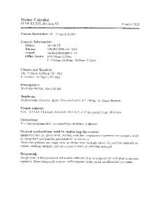
5. The Primal Discrete Vector Calculus In this section, we produce an exact discrete analog of the continuum exact sequence (7). We begin with the description of a simple tensor grid in three-dimensional space. All cell in such grids have rectangular faces. The grid objects are cells, faces, edges, and nodes. As in homology, geometric objects are represented as chains, that is, linear combinations of either cells, faces, edges, or nodes. The boundary of a chain plays an important role and is computed using the boundary operator. Discrete scalar fields are defined on the cells and nodes, while discrete vector fields are defined on the faces and edges. Discrete field are understood to consist of continuum field averages: cell averages of scalar fields associated with the cells, face averages of the normal

10

Nicolas Robidoux, Stanly Steinberg (i,j+1,k+1)

(i,j,k+1)

(i+1,j,k+1)

(i+1,j+1,k+1)

(i,j+1,k)

(i,j,k)

(i+1,j,k)

(i+1,j+1,k)

Generic Cell (i,j+1,k)

(i+1/2,j+1,k)

(i+1,j+1/2,k)

(i,j+1/2,k)

(i+1/2,j,k)

Slice at a Node

(i+1,j+1/2,k+1/2)

(i,j+1/2,k+1/2) (i+1/2,j+1/2,k+1/2)

(i+1/2,j+1/2,k)

(i,j,k)

(i+1/2,j+1,k+1/2)

(i+1,j+1,k)

(i+1,j,k)

(i+1/2,j,k+1/2)

Slice at a Cell Center

Figure 1. Indexing in the Primal Rectangular Grid

components of vector fields associated with the faces, edge averages of the tangential components of vector fields associated with the edges, and point values of scalar fields associated with the nodes. Discrete fields are thus described like chains. The discrete gradient, curl, and divergence are given by simple finite differences. Four integrals are introduced: the integral of a point scalar field over a chain of points, the integral of a edge vector field over a chain of edges, the integral of a face vector field over a chain of faces, and the integral of a cell scalar field over a chain of cells. All of these integrals are simple natural discretizations of Riemann-Stieltjes integrals. These integrals are used to give proofs of the discrete fundamental theorems. The existence of a scalar potential follows the classical argument, but the proof of the existence of a vector potential seems to be novel. We introduce the star operator that connects the primal and dual grids. This is the key to constructing a double exact sequence analog of the continuum double exact sequence (8) and the scalar and vector Laplacians.


11

name part node edge edge edge face face face cell

center

Ni,j,k = {(xi , yj , zk )}

(xi , yj , zk ) xi+ 21 , yj , zk Ei+ 21 ,j,k = {(xi + ξ △x, yj , zk )} xi , yj+ 21 , zk Ei,j+ 21 ,k = {(xi , yj + η △y, zk )} Ei,j,k+ 21 = {(xi , yj , zk + ζ △z)} xi , yj , zk+ 12 xi , yj+ 21 , zk+ 12 Fi,j+ 21 ,k+ 12 = {(xi , yj + η △y, zk + ζ △z)} xi+ 21 , yj , zk+ 12 Fi+ 21 ,j,k+ 21 = {(xi + ξ △x, yj , zk + ζ △z)} Fi+ 21 ,j+ 12 ,k = {(xi + ξ △x, yj + η △y, zk )} xi+ 21 , yj+ 12 , zk xi+ 21 , yj+ 12 , zk+ 12 Ci+ 21 ,j+ 12 ,k+ 12 = {xi + ξ △x, yj + η △y, zk + ζ △z}

orient. + (1, 0, 0) (0, 1, 0) (0, 0, 1) (1, 0, 0) (0, 1, 0) (0, 0, 1) +

Table 2. Geometrical Objects of the Primal Rectangular Grid and their Orientation

5.1. The Tensor Grid The grid is in 3-dimensional Euclidean space R3 and is given by points evenly spaced in each direction, either labeled with an integer or half-integer index. With △x, △y and △z arbitrary positive real numbers, let xi = i △x,

yj = j △y,

zk = k △z,

1 xi+ 1 = (i + ) △x, 2 2

1 yj+ 1 = (j + ) △y, 2 2

1 zk+ 1 = (k + ) △z, 2 2

where −∞ < i, j, k < ∞. The grid is composed of cells C as shown in Figure 1 and the cells are composed of nodes N , edges E, and faces F as describe in Table 2. The parts of the grids are labeled with their midpoints. The variables ξ, η, and ζ are used to parametrize the edges, faces and cells and satisfy 0 6 ξ 6 1, 0 6 η 6 1, 0 6 ζ 6 1. The nodes N of the grid have positive orientation, the edges E are oriented by their unit tangents in the directions of the positive axes, the faces F are are oriented by their unit normals in the directions of the positive axes, and the cells C have positive orientation. 5.2. Chains Volume, surface, and line integral play a central role in vector calculus, but before they can be defined, volumes, surfaces, and curves must be defined. It is convenient to follow the approach used in algebraic topology and differential geometry [36] and define generalized geometric objects called chains. A chain is simply a sum of geometric objects of the same dimension multiplied by a a real number that is the weight for the object. The weight being zero is equivalent to the object not being in the chain, while ±1 gives the orientation of the object. We allow the weights to be in R so that the chains are a linear space. However, it is generally assumed that the chains have compact support, that is, that they have only a finite number of nonzero coefficients. The space of cell chains CC = RC consists of expressions C of the form X (11) C= ai+ 1 ,j+ 1 ,k+ 1 Ci+ 1 ,j+ 1 ,k+ 1 . 2

i,j,k

2

2

2

2

2

12


The space of face chains CF = RF consists of expressions F of the form X X X F = ai,j+ 1 ,k+ 1 Fi,j+ 1 ,k+ 1 + ai+ 1 ,j,k+ 1 Fi+ 1 ,j,k+ 1 + ai+ 1 ,j+ 1 ,k Fi+ 1 ,j+ 1 ,k .

(12)

The space of edge chains CE = RE consists of expressions E of the form X X X ai+ 1 ,j,k Ei+ 1 ,j,k + E= ai,j+ 1 ,k Ei,j+ 1 ,k + ai,j,k+ 1 Ei,j,k+ 1 .

(13)

The space of node chains CN = RN consists of expressions N of the form X N= ai,j,k Ni,j,k .

(14)

2

2

2

2

2

i,j,k

2

2

2

2

i,j,k

2

2

2

2

i,j,k

2

2

i,j,k

2

2

i,j,k

2

i,j,k

i,j,k

5.3. Boundary Operators for Chains The operator that computes the boundary is ∂. For cells, faces, edges, and nodes, the boundaries are: ∂Ci+ 1 ,j+ 1 ,k+ 1 = 2

2

2

Fi+1,j+ 1 ,k+ 1 − Fi,j+ 1 ,k+ 1 + Fi+ 1 ,j+1,k+ 1 − Fi+ 1 ,j,k+ 1 + Fi+ 1 ,j+ 1 ,k+1 − Fi+ 1 ,j+ 1 ,k , 2

2

2

2

2

2

2

2

2

2

2

2

∂Fi,j+ 1 ,k+ 1 = Ei,j+1,k+ 1 − Ei,j,k+ 1 − Ei,j+ 1 ,k+1 + Ei,j+ 1 ,k , 2

2

2

∂F

=E

∂F

=E

i+ 12 ,j,k+ 21 i+ 12 ,j+ 21 ,k

i+ 12 ,j,k+1 i+1,j+ 21 ,k

2

−E

i+ 21 ,j,k

−E

∂Ei+ 1 ,j,k = Ni+1,j,k − Ni,j,k , 2

i,j+ 21 ,k

2

−E

i+1,j,k+ 21

−E

i+ 12 ,j+1,k

2

+ Ei,j,k+ 1 , 2

+E

i+ 12 ,j,k

,

∂Ei,j+ 1 ,k = Ni,j+1,k − Ni,j,k , 2

∂Ei,j,k+ 1 = Ni,j,k+1 − Ni,j,k , 2

∂Ni,j,k = 0. The boundary of a chain is defined by making ∂ linear. Lemma 5.1. ∂∂ ≡ 0. Proof: A direct calculation shows that the boundary of a boundary is empty for cells, faces, and edges. Linearity extends this result to arbitrary chains. 2 5.4. Scalar and Vector Fields Fields have values associated with cells, faces, edges or nodes, with scalar fields having values associated with the nodes and cells and vector fields having values associated with edges and faces. Intuitively, the nodal scalar fields VN correspond to point values of continuum scalar functions, while the cell scalar fields VC correspond to the averages of a continuum scalar field over cells. The edge vector field VE correspond to the average of the tangential component of a continuum vector field over edges, while the face vector field corresponds VF to the average of the normal component of a vector field over faces. It is convenient to represent the fields in terms of a basis, and a natural basis to use is points for scalar fields, edges for edge vector fields, faces for face vector fields and cells for cell scalar fields. In this case chains and fields have exactly the same representation. As


13

with chains, the component of a vector is zero in an expression is equivalent to leaving the corresponding basis element out of the sum. Node: If s ∈ VN then X si,j,k Ni,j,k . (15) s= i,j,k

Edge: If ~t ∈ VE , then X ~t = ti+ 1 ,j,k Ei+ 1 ,j,k + ti,j+ 1 ,k Ei,j+ 1 ,k + ti,j,k+ 1 Ei,j,k+ 1 . 2

2

2

2

2

(16)

2

i,j,k

Face: If ~n ∈ VF , then X ~n = ni,j+ 1 ,k+ 1 Fi,j+ 1 ,k+ 1 + ni+ 1 ,j,k+ 1 Fi+ 1 ,j,k+ 1 + ni+ 1 ,j+ 1 ,k Fi+ 1 ,j+ 1 ,k . 2

2

2

2

2

2

2

2

2

2

2

2

(17)

i,j,k

Cell: If m ∈ VC then

m=

X

mi+ 1 ,j+ 1 ,k+ 1 Ci+ 1 ,j+ 1 ,k+ 1 . 2

2

2

2

2

(18)

2

i,j,k

5.5. Difference Operators The discrete gradient G, curl R and divergence D are defined either by simple differences operating on the coefficients of a field or by their linearity and their values on basis elements. After the definitions, some important analogs of some continuum derivative identities are given. The Gradient: If s ∈ VN is a discrete scalar field, then its gradient Gs ∈ VE is an edge vector field. In terms of components si+1,j,k − si,j,k si,j+1,k − si,j,k si,j,k+1 − si,j,k ; (Gs)i,j+ 1 ,k ≡ ; (Gs)i,j,k+ 1 ≡ , (Gs)i+ 1 ,j,k ≡ 2 2 2 △x △y △z while in terms of the basis elements Ei−1/2,j,k − Ei+1/2,j,k Ei,j−1/2,k − Ei,j+1/2,k Ei,j,−1/2k − Ei,j,k+1/2 GNi,j,k = + + . ∆x ∆y ∆z The Curl: If ~t ∈ VE is a discrete edge vector field, vector field. In terms of components ti,j+1,k+ 1 − ti,j,k+ 1 2 2 (R~t)i,j+ 1 ,k+ 1 ≡ 2 2 △y ti+ 1 ,j,k+1 − ti+ 1 ,j,k 2 2 (R~t)i+ 1 ,j,k+ 1 ≡ 2 2 △z ti+1,j+ 1 ,k − ti,j+ 1 ,k 2 2 (R~t)i+ 1 ,j+ 1 ,k ≡ 2 2 △x

then its curl R~t ∈ VF is a discrete face − − −

ti,j+ 1 ,k+1 − ti,j+ 1 ,k 2

2

△z ti+1,j,k+ 1 − ti,j,k+ 1 2

2

△x ti+ 1 ,j+1,k − ti+ 1 ,j,k 2

2

△y

; ; .

while in terms of basis elements Fi+1/2,j,k+1/2 − Fi−1/2,j,k+1/2 Fi,j+1/2,k+1/2 − Fi,j−1/2,k+1/2 REi,j,k+1/2 = + ∆x ∆y Fi−1/2,j+1/2,k − Fi+1/2,j+1/2,k Fi,j+1/2,k−1/2 − Fi,j+1/2,k+1/2 + REi,j+1/2,k = ∆x ∆z Fi+1/2,j+1/2,k − Fi+1/2,j−1/2,k Fi+1/2,j,k−1/2 − Fi+1/2,j,k+1/2 REi+1/2,j,k = + ∆y ∆z

14


The Divergence: If ~n ∈ VF is a discrete face vector field, then its divergence D~n ∈ VC is a cell scalar field. In terms of components (D~n)i+ 1 ,j+ 1 ,k+ 1 ≡ 2 2 2 ni+1,j+ 1 ,k+ 1 − ni,j+ 1 ,k+ 1 2

2

2

2

△x

+

ni+ 1 ,j+1,k+ 1 − ni+ 1 ,j,k+ 1 2

2

2

2

△y

+

ni+ 1 ,j+ 1 ,k+1 − ni+ 1 ,j+ 1 ,k 2

2

2

2

△z

.

while in terms of basis elements DFi,j+1/2,k+1/2 = DFi+1/2,j,k+1/2 = DFi,j+1/2,k+1/2 =

Ci− 1 ,j+ 1 ,k+ 1 + Ci+ 1 ,j+ 1 ,k+ 1 2

2

2

2

2

2

∆x Ci+ 1 ,j− 1 ,k+ 1 + Ci+ 1 ,j+ 1 ,k+ 1 2

2

2

2

2

2

∆y Ci+ 1 ,j+ 1 ,k− 1 + Ci+ 1 ,j+ 1 ,k+ 1 2

2

2

2

2

, ,

2

∆z A central goal is to show that the discrete differential operators form an exact sequence, just as in the continuum. As part of that goal, a direct computation shows that: Lemma 5.2. Gc ≡ 0,

RG ≡ 0,

DR ≡ 0,

where c is a constant scalar field. 5.6. Integrals Integrals that are natural analogs of the Riemann-Stieltjes integral of fields over cells, faces, edges, or nodes are introduced. As noted above, it is assumed that the chain has compact support. If m ∈ VC as in (18) and C ∈ CC is in (11), then the cell integral of m over C is defined by Z X (19) ai+ 1 ,j+ 1 ,k+ 1 m(i+ 1 ,j+ 1 ,k+ 1 ) △x △y △z. m dV = 2

C

2

2

2

2

2

i,j,k

If ~n ∈ VN as in (17) and F ∈ CF as in (12), then the face integral (of the normal component) of ~n over F is defined by Z X X ~= ai,j+ 1 ,k+ 1 t(i,j+ 1 ,k+ 1 ) △y △z + ~n · dS ai+ 1 ,j,k+ 1 t(i+ 1 ,j,k+ 1 ) △z △x 2

F

2

2

2

2

i,j,k

+

X

2

2

2

i,j,k

ai+ 1 ,j+ 1 ,k t(i+ 1 ,j+ 1 ,k) △x △y. 2

2

2

2

i,j,k

If ~t ∈ VE as in (16) and E ∈ CE as in (13), then edge integral (of the tangential component) of ~t over E is defined by Z X X X ~ = ~t · dL ai,j+ 1 ,k t(i,j+ 1 ,k) △y + ai,j,k+ 1 t(i,j,k+ 1 ) △z. ai+ 1 ,j,k t(i+ 1 ,j,k) △x + E

2

2

2

i,j,k

i,j,k

2

2

2

i,j,k

If f ∈ VN as in (15) and N ∈ CN as in (14), then the integral of f over N is defined by Z X f= ai,j,k fi,j,k . N

i,j,k


15

5.7. The Integral-Derivative Theorems Direct calculations give discrete analogs of the Potential, Stokes’, and Divergence theorems for a single cell, face and edge. Lemma 5.3. If ~n is a face vector field and C is a cell, if ~t is an edge vector field and F is a face, and if f is an nodal scalar field and E is an edge, then Z Z Z Z Z Z ~ ~ = ~ ~= ~t · dL, Gf · dL f. D~n dV = ~n · dS, R~t · dS C

∂C

F

E

∂F

∂E

The next result for general chains follows by linearity:

Theorem 5.1. If C ∈ CC is a cell chain and ~n ∈ VN is a face vector field then Z Z ~ D~n dV = ~n · dS. C

(20)

∂C

If F ∈ CF is a face chain and ~t ∈ VE is a edge vector field then Z Z ~ ~ ~t · dL. ~ Rt · dS = ∂F

F

If E ∈ CE is a edge chain and f VN is a node scalar field then Z Z ~ = Gf · dL f. E

∂E

5.8. The Existence of Potentials If C is a chain and ∂C = 0, then the chain is said to be closed. Similarly, if ~n ∈ VF and D~n ≡ 0, then ~n is said to be closed, if ~t ∈ VE and R~t ≡ 0, then ~t is said to be closed. (A closed node field is constant.) The proofs of the results given below and their implementation in a computer algebra systems are discussed in Appendix A. The first result shows that the if a chain is closed, then it is the boundary of a higher dimensional chain. The proposition is trivial, but plays an important role in building mimetic discretizations. Theorem 5.2. 1. If F ∈ CF has compact support and ∂F = 0, then there is a cell chain C ∈ CC with compact support such that ∂C = F . 2. If E ∈ CE has compact support and ∂E = 0, then there is a face chain F ∈ CF with compact support such that ∂F = E. Theorem 5.3. 1. 2. 3. 4.

If s ∈ VN and Gs ≡ 0 then s is a constant scalar field. If ~t ∈ VE and R~t ≡ 0 then there exists a f ∈ VN such that ~t = Gf . If ~n ∈ VF and D~n ≡ 0 then there exists a ~t ∈ VE such that ~n = R~t. For any m ∈ VC , there exists ~n ∈ VF such that D~n = m.

5.9. A Mimetic Vector Calculus The previous results imply that the following sequence is exact, and conversely, the fact that the sequence is exact summarizes the previous results. G

R

D

R −−−→ VN −−−→ VE −−−→ VF −−−→ VC −−−→ 0. This produces a mimetic vector calculus.

16


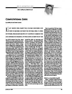
(i−1/2,j+3/2,k+3/2)

(i−1/2,j+1/2,k+3/2)

(i+1/2,j+1/2,k+3/2)

(i+1/2,j+3/2,k+3/2)

(i,j,k+1)

(i+1/2,j+3/2,k+1/2) (i,j+1,k)

(i,j,k)

(i+1,j,k)

(i+1,j+1,k) Figure 2. The Primal and Dual Grid Cells

5.10. The Dual Grid Unlike the continuum, the codomain of G is not the same space as the domain of D, so something additional needs to be done to define the scalar Laplacian DG. In addition, the codomain of R is not the same as the domain of R, so something additional is also needed to define the vector Laplacian RR. A classical solution to this problem is to introduce averaging operators between the spaces VN and VC , and between the spaces VE and VF . Unfortunately, averaging operators are generally not invertible. We use another classical way of resolving the mismatch: a dual grid. All dual grid objects are labeled with a star. As shown in Figure 2, the dual grid is obtained by translating the primal grid by (∆x/2, ∆y/2, ∆z/2) so that nodes correspond to cell centers and edge centers correspond to face centers. The edges in the grid pass perpendicularly through the centers of the dual grid faces and vice versa. Because the dual grid is a translate of the primal grid, all the primal calculus results hold for the dual grid. See Appendix B for details.


17

5.11. The Star Operator The geometric ⋆ operator is a bijection that associates the following objects: ⋆ ⋆Ni,j,k = Ci,j,k ,

⋆ , ⋆Ei+ 1 ,j,k = Fi+ 1 ,j,k 2

2

⋆ ⋆Ci+ 1 ,j+ 1 ,k+ 1 = Ni+ 1 ,j+ 1 ,k+ 1 2

2

2

2

2

2

⋆ ⋆Fi,j+ 1 ,k+ 1 = Ei,j+ , 1 ,k+ 1

··· ,

2

2

2

2

··· .

The inverse of this map is also labeled with ⋆. Matching indices also defines bijections between primal and dual fields: ⋆ = ⋆(N,C ⋆ ) : VN → VC ⋆ , m⋆i,j,k = ⋆fi,j,k = fi,j,k ,   n⋆ = ⋆ti+ 1 ,j,k = ti+ 1 ,j,k ,  2 2  i+ 21 ,j,k ⋆ 1 n = ⋆t = t ⋆ = ⋆(E,F ⋆ ) : VE → VF ⋆ , i,j+ 2 ,k i,j+ 21 ,k , i,j+ 21 ,k   n⋆ = ⋆ti,j,k+ 1 = ti,j,k+ 1 , i,j,k+ 21 2 2  ⋆  t = ⋆ni,j+ 1 ,k+ 1 = ni,j+ 1 ,k+ 1 ,  2 2 2 2  i,j+ 21 ,k+ 21 ⋆ 1 1 1 1 t = ⋆n = n ⋆ ⋆ = ⋆(F,E ⋆ ) : VF → VE , i+ 2 ,j,k+ 2 i+ 2 ,j,k+ 2 , i+ 21 ,j,k+ 21   t⋆ 1 1 = ⋆n 1 1 = n 1 1 , i+ 2 ,j+ 2 ,k

i+ 2 ,j+ 2 ,k

i+ 2 ,j+ 2 ,k

⋆ ⋆ = ⋆(C,N ⋆ ) : VC → VN ⋆ , fi+ = ⋆mi+ 1 ,j+ 1 ,k+ 1 = mi+ 1 ,j+ 1 ,k+ 1 , 1 ,j+ 1 ,k+ 1 2

2

2

2

2

2

2

2

2

(21)

with ⋆(C ⋆ ,N ) = ⋆−1 (N,C ⋆ ) ,

⋆(F ⋆ ,E) = ⋆−1 (E,F ⋆ ) ,

⋆(E ⋆ ,F ) = ⋆−1 (F,E ⋆ ) ,

⋆(N ⋆ ,C) = ⋆−1 (C,N ⋆ ) ,

so that ⋆2 = ⋆ ⋆ is the identity. In the present article, only the simplest star operators—those with ”identity matrix” representations with respect to cardinal bases—are considered. In order to get higher order accuracy on non-uniform grids and/or with nontrivial material properties, more complex, generally non-diagonal, star operators must be used. 5.12. The Double Exact Sequence The operators on the dual grid are like the operators on the primal grid save for a change of notation. So there is both an exact sequence (8) and a dual exact sequence. They are related by the ⋆ operator: G

R −−−→ VN −−−→   ⋆y D⋆

R

VE −−−→   ⋆y R⋆

D

VF −−−→   ⋆y G⋆

VC −−−→ 0   ⋆y

0 ←−−− VC ⋆ ←−−− VF ⋆ ←−−− VE ⋆ ←−−− VN ⋆ ←−−− R

Theorem 5.4. Both sequences in (22) are exact and the ⋆ operators are bijective.

(22)

18


5.13. The Laplacians Each square of the above double exact sequence, traversed in the clockwise direction, defines a discrete Laplacian. Starting with the spaces in the primal exact sequence gives the primal scalar and vector Laplacians, as well as a third operator found in the literature but which does not appear to have a name. When the meaning is clear, the second-order operators are written without explicitly showing star operators: L = D ⋆ G = ⋆D ⋆ ⋆ G ≡ ⋆(C ⋆ ,N ) D ⋆ ⋆(E,F ⋆ ) G, ~ = R⋆ R = ⋆R⋆ ⋆ R ≡ ⋆(F ⋆ ,E)R⋆ ⋆(F,E ⋆ ) R, L L¯ = G ⋆ D = ⋆G ⋆ ⋆ D ≡ ⋆(E ⋆ ,F )G ⋆ ⋆(C,N ⋆ ) D,

on VN ,

(23)

on VE , on VF .

(24) (25)

Starting with the spaces in the dual exact sequence produces a conjugate set of second-order ¯ on VE ⋆ . ~ on VF ⋆ and G ⋆ ⋆ D⋆ = ⋆L⋆ operators: D ⋆ ⋆ G⋆ = ⋆L⋆ on VC ⋆ , R⋆ ⋆ R⋆ = ⋆L⋆ 5.14. Summary We now have the tools to produce spatial discretizations of the partial differential equations that appear in continuum mechanics. Many of the details in this section were checked in the Mathematica notebooks Discrete.nb and PrimaryGrid.nb.

6. Analysis of the Laplacians In this section, we show that the scalar Laplacian is negative and the vector Laplacian is positive, critical results for analyzing boundary value problems involving these operators. It is important to understand that the material in this section is not directly used in the algorithms using mimetic ideas; the material is used to analyze the algorithms. The analysis depends critically on the vector integration by parts theorems: the Stokes’ and Divergence theorems. These in turn, depend on the definitions of scalar and vector products. Defining these products is straight forward if a bit complicated. Importantly, the wedge product used in differential geometry (see §C.1) provides strong constraints on what products should be defined. We have also found that we only need to define products between primal and dual fields. But before any of this can be done, we need to be able to add and multiply discrete fields. 6.1. Universal Averaging and Sums and Products of Fields In the continuum, scalar fields and vector fields are added by adding their values at the same physical point. The same holds true for scalar, cross and dot products. For addition, the fields also must have the same units. So for example, adding t and n⋆ is not allow even though they are defined at the same points. However, it is OK to add t and ⋆n⋆ . To compensate for the grid staggering, we introduce the universal averaging operator µ. To obtain the value of a discrete field at a point where it is not defined, the operator µ averages the values of the field at the logically nearest neighbors where the field is defined. In many cases it is not necessary to explicitly write µ. For example, if f is a primal scalar field, then fi,j,k + fi+1,j,k 2 fi,j,k + fi+1,j,k + fi,j+1,k + fi+1,j+1,k . = 2

µ(f )i+ 1 ,j,k = fi+ 1 ,j,k = 2

2

µ(f )i+ 1 ,j+ 1 ,k = fi+ 1 ,j+ 1 ,k 2

2

2

2


1 2 3 4 5 6 7 8 9 10

19

f m⋆ : VN × VC ⋆ → VC ⋆ , f ~n⋆ : VN × VF ⋆ → VF ⋆ , f ~t⋆ : VN × VE ⋆ → VE ⋆ , f f ⋆ : VN × VN ⋆ → VN ⋆ , ~t · ~n⋆ : VE × VF ⋆ → VC ⋆ ,

f ⋆ m : VN ⋆ × VC → VC , f ⋆ ~n : VN ⋆ × VF → VF , f ⋆ ~t : VN ⋆ × VE → VE , f ⋆ f : VN ⋆ × VN → VN , ~t⋆ · ~n : VE ⋆ × VF → VC ,

~t × ~t⋆ : VE × VE ⋆ → VF ⋆ , ~t f ⋆ : VE × VN ⋆ → VE ⋆ , ~n · ~t⋆ : VF × VE ⋆ → VC ⋆ ,

~t⋆ × ~t : VE ⋆ × VE → VF , ~t⋆ f : VE ⋆ × VN → VE , ~n⋆ · ~t : VF ⋆ × VE → VC ,

~n f ⋆ : VF × VN ⋆ → VF ⋆ , m f ⋆ : VC × VN ⋆ → VC ⋆ ,

~n⋆ f : VF ⋆ × VN → VF , m⋆ f : VC ⋆ × VN → VC .

Table 3. Products of Vectors and Scalars. (Definitions are given in Appendix C.3.)

More formulas are given in Appendix C.2. It is important that the universal averaging operator is not used to define the second-order differential operators, only to analyze them. 6.2. Scalar and Vector Products of Fields We now construct discrete analogs of the continuum scalar and vector products that are listed in (10). The definitions of the discrete products is complicated by the grid staggering and by the use of dual grids, which leads to some large formulas recorded in Appendix C.3. The discrete star operator is used to reduce the possible products to those between elements of the primal and dual fields. Table 3 enumerates the possibilities. Note that the products are defined for objects in different spaces, so that it does not make sense to ask if they commute or anti-commute. Also, there are still two possibilities for the range of a product. We have chosen the convention that the product of a and b ends up in the same space as b. For example, for the formula (26), we use the definitions: f ~n⋆ : VN × VF ⋆ → VF ⋆ , (f ~n⋆ )i+ 1 ,j,k = µ(f )i+ 1 ,j,k n⋆i+ 1 ,j,k , 2

⋆

⋆

f m : VN × VC ⋆ → VC ⋆ , (f m )i,j,k = ~t · ~n : VE × VF ⋆ → VC ⋆ , (~t · ~n )i,j,k = ⋆

⋆

+

2

2

fi,j,k m⋆i,j,k , ti− 1 ,j,k n⋆i− 1 ,j,k 2 2

+ ti+ 1 ,j,k n⋆i+ 1 ,j,k 2

ti,j− 1 ,k n⋆i,j− 1 ,k + ti,j+ 1 ,k n⋆i,j+ 1 ,k 2

2

2

2

2

2

2

+

ti,j,k− 1 n⋆i,j,k− 1 + ti,j,k+ 1 n⋆i,j,k+ 1 2

2

2

2

2

.

Dot products are only defined for vectors that are located at the same points in the grid (also see (47) and (48)), so the dot product is given by multiplying the co-located values and then averaging the result to a cell center in the primal or dual grid. Cross products are a bit more difficult, but geometrically natural. For example, consider ~t⋆ × ~t from the second column of row 9 of Table 3, for which the formula is given in (50). This is a cell-face quantity in the primary grid of which the x component is ~t⋆ × ~t . i,j+ 1 ,k+ 1 2

2

20


This quantity involves the product of the y component of ~t⋆ and the z component of ~t minus the product of the z component of ~t⋆ times the y component of ~t (see C.1). The first of these two terms thus involves the two quantities t⋆i+ 1 ,j,k+ 1 and ti,j,k+ 1 . 2

2

2

To multiply these two terms they have to be at the same point, so we first average t⋆ to get the quantity t⋆i− 1 ,j,k+ 1 + t⋆i+ 1 ,j,k+ 1 2 2 2 2 Q1i,j,k+ 1 = ti,j,k+ 1 . 2 2 2 However, this quantity is located on an edge of the face on which we are defining ~t⋆ × ~t, so we average this quantity on the two parallel edges to get Q2i,j+ 1 ,k+ 1 = 2

Qi,j,k+ 1 + Qi,j+1,k+ 1 2

2

2

2

.

Q2 is the desired term. The remaining terms in the formula can be computed similarly. Details are found in the notebook Conservation.nb. 6.3. Divergence of Products Identities We are now ready to prove discrete analogs of the continuum divergence identities (9). Theorem 6.1. D ⋆ (f ~n⋆ ) = f D ⋆ (~n⋆ ) + G(f ) · ~n⋆ , D(f ⋆ ~n) = f ⋆ D(~n) + G ⋆ (f ⋆ ) · ~n, D ⋆ (~t × ~t⋆ ) = R~t · ~t⋆ − ~t · R⋆~t⋆ , D(~t⋆ × ~t) = R⋆~t⋆ · ~t − ~t⋆ · R~t,

in VC ⋆ , in VC ,

(26) (27)

in VC ⋆ ,

(28)

in VC .

(29)

Proof: The notebook Conservation.nb provides details of the proofs by direct computation. Because the range of D ⋆ is VC ⋆ , the first identity means D ⋆ (f ~n⋆ )(i,j,k) = (f D ⋆ (~n⋆ ))(i,j,k) + (G(f ) · ~n⋆ )(i,j,k) (see (41), (39) and (47)). The second identity must be verified at (i + 1/2, j + 1/2, k + 1/2) because it holds in VC (see (42), (40) and (48)). The third identity must be verified at (i, j, k) because it holds in VC ⋆ (see (50), (51) and (47)). Finally, the fourth identity must be verified at (i + 1/2, j + 1/2, k + 1/2) because it holds in VC (see (49), (52) and (48)). 2 6.4. Bilinear Forms and Duality When two spaces in the double exact sequence (22) are connected by a vertical arrow, the elements of the spaces have the same indices, that is, they are defined at the same spatial point. Consequently, there are four natural bilinear forms all of which are labeled with B. The constant area unit △x△y△z is introduced to make it easier to interpret the bilinear forms as integrals. Throughout, we assume that one of the fields in the bilinear form has compact support.


21

Node-Cell Bilinear Form: If f ∈ VN and m⋆ ∈ VC ⋆ , then X B(f, m⋆ ) = fi,j,k m⋆i,j,k △x△y△z.

(30)

i,j,k

Edge-Face Bilinear Form: If ~t ∈ VE and ~n⋆ ∈ VF ⋆ , then X ti+ 1 ,j,k n⋆i+ 1 ,j,k + ti,j+ 1 ,k n⋆i,j+ 1 ,k + ti,j,k+ 1 n⋆i,j,k+ 1 △x△y△z. B(~t, ~n⋆ ) =

(31)

Face-Edge Bilinear Form: If ~n ∈ VF and ~t⋆ ∈ VE ⋆ , then   ni,j+ 1 ,k+ 1 t⋆i,j+ 1 ,k+ 1 2 2 2 2 X  ⋆ B(~n, ~t⋆ ) =  + ni+ 21 ,j,k+ 21 ti+ 12 ,j,k+ 21  △x△y△z. i,j,k + ni+ 1 ,j+ 1 ,k t⋆i+ 1 ,j+ 1 ,k

(32)

2

2

2

i,j,k

2

2

2

2

2

2

2

⋆

Cell-Node Bilinear Form: If m ∈ VC and f ∈ VN ⋆ , then X ⋆ B(m, f ⋆ ) = mi+ 1 ,j+ 1 ,k+ 1 fi+ △x△y△z. 1 ,j+ 1 ,k+ 1 2

2

2

i,j,k

2

2

2

(33)

Because the fields in the above definitions are located at the same points, B(⋆m⋆ , ⋆f ) = B(f, m⋆ ), B(⋆f ⋆ , ⋆m) = B(m, f ⋆ ), B(⋆~n⋆ , ⋆~t) = B(~t, ~n⋆ ), B(⋆~t⋆ , ⋆~n) = B(~n, ~t⋆ ). Lemma 6.1. The pairs of spaces VN and VC ⋆ ,

VE and VF ⋆ ,

VF and VE ⋆ ,

VC and VN ⋆ ,

are dual under the non-degenerate bilinear form B. That is, the fields with compact support in one space are non-degenerate linear functionals on arbitrary fields in the dual space. Under the assumption that one of the fields has compact support, an integral without domain of integration is performed over the full grid. With this notation, the above bilinear forms can be written with familiar notation: Lemma 6.2. Each of the four bilinear forms (30)–(33) has two representations: Node-Cell Bilinear Form: Z Z ⋆ ⋆ B(f, m ) = m f dV = f m⋆ dV ⋆ ;

(34)

Cell-Node Bilinear Form: ⋆

f m dV =

Z

m f ⋆ dV ⋆ ;

(35)

Z

~n · ~t dV =

Z

~t · ~n⋆ dV ⋆ ;

(36)

Z

~⋆

Z

~n · ~t⋆ dV ⋆ .

(37)

B(m, f ) =

Z

⋆

Edge-Face Bilinear Form: B(~t, ~n ) = ⋆

⋆

Face-Edge Bilinear Form: ~⋆

B(~n, t ) =

t · ~n dV =

22


Proof: The key point is that the sum over all the grid of the average of a field is the average of the sum, which is just the sum. For the Node-Cell case, m⋆ f is defined in (54) as an average, while f m⋆ is defined in (39) and does not need an average. So Z X m⋆ f dV = (m⋆ f )i+ 1 ,j+ 1 ,k+ 1 dx dy dz 2 2 2   ⋆ (m f )i,j,k + (m⋆ f )i+1,j,k X 1  + (m⋆ f )i,j+1,k + (m⋆ f )i,j,k+1   dx dy dz  = 8  + (m⋆ f )i,j+1,k+1 + (m⋆ f )i+1,j,k+1  + (m⋆ f )i+1,j+1,k + (m⋆ f )i+1,j+1,k+1 X X = (m⋆ f )i,j,k dx dy dz = (f m⋆ )i,j,k dx dy dz = B(f, m⋆ ) and

Z

f m⋆ dV ⋆ dV ⋆ =

X

(f m⋆ )i,j,k dx dy dz = B(f, m⋆ ).

The remaining cases are similar. For the Cell-Node case, f ⋆ m is defined in (40) and doesn’t require an average, while m f ⋆ is defined in (53) and needs an average. For the Edge-Face case, ~n⋆ ~t is defined in (52) as an average, and ~t ~n⋆ is defined in (47) and also requires an average. For the Face-Edge case ~t⋆ ~n is defined in (48) as an average, and ~n ~t⋆ is defined in (51) and also requires an average. (Details are given in the notebook Conservation.nb.) 2 6.5. Duality of the Vector Differential Operators The next result is critical for understanding the Laplacian operators. Theorem 6.2. The pairs of operators G and D ⋆ , D and G ⋆ , and R and R⋆ , are ± duals of each other in the bilinear form B: B(f, D ⋆~n⋆ ) + B(Gf, ~n⋆ ) = 0,

B(D~n, f ⋆ ) + B(~n, G ⋆ f ⋆ ) = 0,

B(R~t, ~t⋆ ) − B(~t, R⋆~t⋆ ) = 0. (38)

where at least one of the fields in the bilinear form has compact support. Proof: The proofs consist of integrating product rule identities over the whole grid. For the first identiry, integration of (26) gives Z Z Z ⋆ ⋆ ⋆ ⋆ ⋆ ⋆ D (f ~n ) dV = f D (~n ) dV + G(f ) · ~n⋆ dV ⋆ . So the dual of the Divergence theorem (20) and the compact support gives that the left-hand side is zero. (34) and (36) complete the computation. Integration of (27) gives Z Z Z ⋆ ⋆ D(f ~n) dV = f D(~n) dV + G ⋆ (f ⋆ ) · ~n dV,

where the integral is given in(19). So the Divergence theorem (20) and the compact support gives that the left-hand side is zero. Then, (35) and (37) give the result. Integration of (28) gives Z Z Z ⋆ ~ ⋆ ⋆ ⋆ ⋆ ~ ~ ~ D (t × t ) dV = Rt · t dV − ~t · R⋆~t⋆ dV ⋆ . So the dual of the Divergence theorem (20), discussed in Appendix B, and the compact support gives that the left-hand side is zero. Then, (37) and (36) give the result. 2


23

6.6. Inner Products and Laplacians The bilinear forms (34), (35), (36) and (37) induce inner products on the compactly supported fields in discrete primal and dual spaces. For the primal case: hf1 , f2 i = B(f1 , ⋆f2 ), ∀f1 , f2 ∈ VN , h~t1 , ~t2 i = B(~t1 , ⋆~t2 ), ∀~t1 , ~t2 ∈ VE , h~n1 , ~n2 i = B(~n1 , ⋆~n2 ), ∀~n1 , ~n2 ∈ VF , hm1 , m2 i = B(m1 , ⋆m2 ), ∀m1 , m2 ∈ VN . For the dual case: hf1⋆ , f2⋆ i = B(⋆f1⋆ , f2⋆ ), ∀f1⋆ , f2⋆ ∈ VN ⋆ , h~t⋆1 , ~t⋆2 i = B(⋆~t⋆1 , ~t⋆2 ), ∀~t⋆1 , ~t⋆2 ∈ VE ⋆ , h~n⋆1 , ~n⋆2 i = B(⋆~n⋆1 , ~n⋆2 ), ∀~n⋆1 , ~n⋆2 ∈ VF ⋆ , hm⋆1 , m⋆2 i = B(⋆m⋆1 , m⋆2 ), ∀m⋆1 , m2 ∈ VN ⋆ . Their related norms are k · k2 = h·, ·i. In fact, these inner products are the standard finitedimensional mean-square inner products multiplied by the cell area. Note that the symmetry can be seen from, for example, hf1 , f2 i = B(f1 , ⋆f2 ) = B(⋆ ⋆ f2 , ⋆f1 ) = B(f2 , ⋆f1 ) = hf2 , f1 i. Lemma 6.3. The operators − ⋆ D ⋆ ⋆ G (23), − ⋆ G ⋆ ⋆ D (25) and ⋆R⋆ ⋆ R (24) are symmetric and positive. Proof: The adjoint relationships (38) give: h⋆D ⋆ ⋆ Gf1 , f2 i = B(⋆D ⋆ ⋆ Gf1 , ⋆f2 ) = B(f2 , D ⋆ ⋆ Gf1 ) = −B(Gf2 , ⋆Gf1 ) = −hGf2 , Gf1 i; h⋆G ⋆ ⋆ D~n1 , ~n2 i = B(⋆G ⋆ ⋆ D~n1 , ⋆~n2 ) = B(~n2 , G ⋆ ⋆ D~n1 ) = −B(D~n2 , ⋆D~n1 ) = −hD~n2 , D~n1 i; h⋆R⋆ ⋆ R~t1 , ~t2 i = B(⋆R⋆ ⋆ R~t1 , ⋆~t2 ) = B(~t2 , R⋆ ⋆ R~t1 ) = B(R~t2 , ⋆R~t1 ) = hR~t2 , R~t1 i. This implies that h− ⋆ D ⋆ ⋆ Gf, f i = kGf k2 ;

h− ⋆ G ⋆ ⋆ D~n, ~ni = kD~nk2 ;

h⋆R⋆ ⋆ R~t, ~ti = kR~tk2 . 2

~ ∇× ~ −∇ ~ ∇· ~ plays an important role in differential geometry. A The Hodge Laplacian ∇× ⋆ discrete analog of this operator is ⋆R ⋆ R − G ⋆ D ⋆ ⋆. Lemma 6.4. The Hodge Laplacian is symmetric and positive. Proof: hG ⋆ D ⋆ ⋆ ~t1 , ~t2 i = B(G ⋆ D ⋆ ⋆ ~t1 , ⋆~t2 ) = −B(⋆D ⋆ ⋆ ~t1 , D ⋆ ⋆ ~t2 ) = hD ⋆ ⋆ ~t1 , D ⋆ ⋆ ~t2 i. Combining this with the second formula in the previous proof gives ~ ∇× ~ −∇ ~ ∇· ~ ~t, ~ti = kR~tk + kD ⋆ ⋆ ~tk2 . 2 h∇×

24


7. Future Directions The many ongoing research projects relying on mimetic methods to solve varied applied modeling problems prove that discrete conservation laws/integration identities lead to robust and accurate numerical methods. What is not so clear is the following: Can mimetic methods solve problems significantly better—more accurately, cheaply, and/or with reduced programming effort—than comparably sophisticated mixed finite element methods [33] and finite volume methods [44]? An affirmative answer to this question requires that a mimetic method produce, for an important problem, a numerical solution of a quality unattainable with alternative methods. Such a “closer” is likely to consist of the successful solution of a problem with one or more of the following features: • Rough solutions or coefficients, leading to highly non-classical solutions. • Unusual boundary conditions leading, for example, to non-coercive bilinear forms. • Unstable problems, or blow up solutions, about which accurate averaged or asymptotic properties are desired. • Problems better formulated in term of tensors, that is, problems for which vector calculus is insufficiently expressive. Problems with singular, degenerate, or rapidly varying material properties or solutions may provide problems that non-mimetic methods fail to solve satisfactorily. (General relativity comes to mind.) Somewhat related is the problem of computing effective (averaged) properties for complex materials (homogenization theory), a promising field of application of mimetic principles. In other words, it may be that mimetic methods end up being a preferred method because of their compatibility with the macroscopic modeling of material properties. To our knowledge, a “killer” mimetic application has yet to be found. For this reason, it is still unclear whether mimetic discretizations will be seen as superior alternatives to finite element and finite volume methods, or whether mimetic properties will eventually come to be seen as important features of high quality methods derived without explicitly using mimetic discretization methods. In other words, the jury is still out regarding whether mimetic discretization methods will survive as a full-fledge derivation, or will be a footnote to the slow convergence of finite element and finite volume methods. On the other hand, mimetic ideas may turn out to be a unifying principle for a number of finite difference, finite volume and finite element methods. In the remainder of this section, we list a few promising, more theoretical, research directions. Logically rectangular, but not tensor, grids, that is, grids with “deformed” cells, have received a lot of attention. If the grid is smooth, mapping methods can be used to carry approximations on tensor grids over to the deformed grid without too great an accuracy loss. Mapping methods, however, do not perform well when the grid is not smooth. Furthermore, topological complications arise if the grid is only piecewise logically rectangular. A definitive treatment of rough grids and complex grid topologies is needed. A promising research avenue concerns the development of (piecewise) spectral and pseudospectral methods that do not lose their rapid convergence when the solution, or the grid, is not smooth everywhere, in other words, the use of mimetic principles to stabilize high order approximations.


25

Mixed linear or nonlinear boundary conditions in higher dimensions also deserve further study. The linear 1D case was fully treated in [122], but matters are complicated in higher dimensions, especially if the boundary conditions involve field components other than those which appear in the appropriate version of Stokes’ Theorem. Also left out of the present paper is the issue of time discretization. The Finite Difference Time Domain method suggests the use of grids staggered in both time and space [152]. Consider, for example, the scalar wave equation written as a first order system: ∂f ~ v, = ∇·~ ∂t

∂~v ~ . = ∇f ∂t

Taking cues from relativity theory, treat time as “just another” spatial variable: Letting f = f (t, x, y, z) , set f =

~v = (v0 , v1 , v2 , v3 ) with vi = vi (t, x, y, z) ,

∂f ∂f ∂f ∂f , , , ∂t ∂x ∂y ∂z

,

and · ~v =

∂v0 ∂v1 ∂v2 ∂v3 + + + . ∂t ∂x ∂y ∂z

Then, if A is the 4×4 diagonal matrix with diagonal equal to (−1, 1, 1, 1), · Af = 0 is the wave equation. The space-time divergence · is the key to fully discrete conservation laws. Following the ideas used in the time-independent case, natural discretizations of · and on staggered grids can be obtained. The question now becomes: how can one construct analogs of the matrix A leading to accurate solutions of the wave equation. The current paper assumes a rectangular data structure. Triangular/tetrahedral data structures, however, are extremely important. Mimetic methods have been implemented on triangular and tetrahedral grids and these methods work well. With some major changes, the theory presented in the present paper is applicable to this situation: In terms of a master element, a dual grid can be generated by connecting the barycenter of the triangle/tetrahedron to the centers of the sides/faces of the triangle. This leads to auxiliary values on the sides/faces of the triangles. If the side/face turns is in the interior of the region, the corresponding auxiliary value can be eliminated; If the side/face is on the boundary of the region, the corresponding auxiliary value can be used in the discretization of the boundary conditions. Major complications arise from the fact that the topology of a simplicial grid can be considerably more complex than the topology of a logically rectangular one. Numerical Hodge-Helmholtz decompositions needs refinement and additional flexibility. The connection between geometric integration and mimetic discretization methods deserves investigation. There simply must be be a link between the preservation of Lie-Poisson brackets, generally obtained by integration by parts [108], and mimetic summation-by-parts formulas. Yet, the two fields have evolved without much cross-pollination. This may be because the early development of geometric integration focused on discretizing systems of ordinary differential equations, with special emphasis on the preservation of antisymmetric bilinear forms (and Hamiltonian structures) [107], while the development of many mimetic discretization methods started with the diffusion equation, with an emphasis on preserving symmetric bilinear forms. Mimetic discretizations based on discrete Hodge star operators constructed with Whitney map reconstruction and deRham projection generally assume one single primal/dual

26


grid pair. A powerful generalization involves the averaging of Hodge star operators over parameterized families of dual grids. For example, if the steady-state diffusion equation ~ ~ −∇·(K ∇u) = 0 is discretized with a fixed primal (cell) grid but a parameterized family of dual grids obtained by linearly varying the position of the dual nodes within the cells (using, in triangular cells, barycentric coordinates), the Galerkin Hodge star is exactly recovered by averaging when the diffusion coefficient matrix K is constant within each cell. On the other hand, the Galerkin Hodge star is only approximately recovered when K varies within each cell. (In 1D, the averaged and and the Galerkin discrete Hodge are the same irregardless of whether or not the diffusion coefficient is constant.) If one could devise a method of constructing the parameterized family of dual grids from the primal, and a matching method of averaging Hodge star operators, which automatically produces the Galerkin discrete Hodge star, this would link the finite element approach toward discretizing material properties (by way of bilinear forms) with the “direct” approach advocated, among others, by Claudio Mattiussi [101, 103], following the work of Enzo Tonti [141, 142]. It would also lead to Whitney-deRham Hodge stars with symmetric matrix representations, a desirable feature from a practical viewpoint. (Note that there is a mild abuse of terminology in the above discussion, since the discrete Hodge star is taken as containing both metric and material property information, a proposition which should not surprise the general relativists in the audience.) A final note: Currently, there is no user-friendly (in Matlab or Scilab, say) general purpose numerical software implementing mimetic methods. This is not surprising given that a general yet unified “standard” mimetic discretization theory does not exist. The availability of such software would go a long way toward popularizing the framework, as it would allow researchers to experiment with established and novel mimetic formulations without too high an initial programming investment.

A. The Existence of Potentials Proof of Theorem 5.2, part 1: Basically, we collapse the face chain toward k = 0, at which point it must be trivial. Let F be a face chain with compact support and ∂F = 0. Without loss of generality, suppose that F 6= 0 (otherwise, take C = 0) and that the indices of nonzero coefficients of F are non-negative. Let K be the maximum value of all the third indices (full or half) of the nonzero faces of F . We assert that K must be an integer (not a half-integer). Otherwise, the maximum can be written K = k + 12 with k an integer. There are four possibilities: Fi+ 1 ,j,k+ 1 , Fi− 1 ,j,k+ 1 , Fi,j+ 1 ,k+ 1 and Fi,j− 1 ,k+ 1 for some integers i and j. Let us consider the 2 2 2 2 2 2 2 2 first possibility (the other three are similar). The boundary of the face Fi+ 1 ,j,k+ 1 contains 2 2 the edge Ei+ 1 ,j,k+1. This edge is part of only three other faces: Fi+ 1 ,j+ 1 ,k+1 , Fi+ 1 ,j− 1 ,k+1, 2 2 2 2 2 and Fi+ 1 ,j,k+ 3 . For the boundary of the chain to be zero, the chain must contain a face other 2 2 than the last, contradicting the assumption that K is maximal. Now, construct the cell chain C with ∂C = F . Start by setting C = 0. Choose any face in F of the form Fi± 1 ,j± 1 ,K . By linearity, assume that its coefficient is 1. F is in the boundary 2 2 of the cell Ai± 1 ,j± 1 ,K− 1 . Now set C = C + Ai± 1 ,j± 1 ,K− 1 and F = F − ∂Ai± 1 ,j± 1 ,K− 1 . Note 2 2 2 2 2 2 2 2 2 that the new F still satisfies ∂F = 0 (because ∂ 2 = 0) and that there is only one face with maximal k index in the boundary of Ai± 1 ,j± 1 ,K− 1 . This is important, because this implies 2 2 2 that we have “removed” one face with maximal index and that the only other faces with coefficients affected by this step have smaller third indices. Note also that these affected


27

faces have third index equal to K − 21 or K − 1. For this reason, we can continue until the largest third index is 0, which means that all the third indices of the remaining face are equal to 0. As discussed above, the only way we can get ∂F = 0 is by having a face with half-integer third index in the chain. Since there are none, all the coefficients of the final face must be zero, which implies that the initial face is the boundary of the final cell. The final cell chain C has compact support because at most one cell is added per step, and this algorithm terminates. (This algorithm was implemented in the notebook InverseOfBoundary.nb.) 2 Proof of Theorem 5.2, part 2: The procedure first collapses all third indices toward zero, at which point the remaining edge chain must be trivial. Let E be an edge chain with compact support and ∂E = 0. Without loss of generality, suppose that E 6= 0 and that all its nonzero cofficients have non-negative third index. Edges in E have the form Ea,b,c where one and only one of a, b and c is a half-integer. Find the maximum value of c over the edges with nonzero coefficients, and choose a corresponding edge Ea,b,c with nonzero coefficient. By linearity, assume the coefficient to be 1. The maximal third index c cannot be a half-integer because otherwise one of its endpoints would have a third index larger than c, which implies that an edge with a larger third index would have to be in E in order for ∂E to vanish. Consequently, Ea,b,c = Ea,b,K with K an integer. Ea,b,K is in the boundary of Fa,b,K− 1 . Add this face to the chain F being constructed 2 and remove its boundary from E. The new E is still closed. In addition, Ea,b,K is the only face with maximal third index which is affected, and the third indices of the other affected edges are K − 12 and K − 1. For this reason, we can continue until the maximal third index is 0, which means that the third index of every remaining edge is 0. Now, consider the maximal second index of the nonzero coefficients of the remaining edge chain. This maximal second index must be an integer. However, the third index is 0. Since edges cannot have two integer indices, we must have that there were no nonzero coefficients. This implies that the boundary of the final face is the initial edge. The final F has compact support because the algorithm terminates. (This algorithm was implemented in the notebook InverseOfBoundary.nb.) 2 Proof of Theorem 5.3, part 1: This is a direct calculation. Its converse was noted earlier. Proof of Theorem 5.3, part 2: Except for the fact that are integrals and paths are discrete, this is the classical proof based on the fact that the integral of the tangential component of a closed vector field ~t is path independent. 2 Proof of Theorem 5.3, part 3: As all cells are translates of each other, it is enough to consider C 1 , 1 , 1 . On this cell the divergence condition implies that the given face vector field must 2 2 2 satisfy n 1 ,1, 1 − n 1 ,0, 1 n 1 , 1 ,1 − n 1 , 1 ,0 n1, 1 , 1 − n0, 1 , 1 2 2 2 2 2 2 2 2 + 2 2 + 22 = 0, △x △y △z while the desired edge vector field is given by the twelve values t0,0, 1 , t0, 1 ,0 , t0, 1 ,1 , t1,0, 1 , t1,1, 1 , 2 2 2 2 2 t1, 1 ,0 , t1, 1 ,1 , t 1 ,0,0 , t 1 ,0,1 , t 1 ,1,0 and t 1 ,1,1 . These must satisfy 2

2

2

n0, 1 , 1 = + 2 2

n 1 ,0, 1 = + 2

2

n 1 , 1 ,0 = + 2 2

2

2

2

t0,1, 1 − t0,0, 1 2

2

△y t 1 ,0,1 − t 1 ,0,0 2

2

△z t1, 1 ,0 − t0, 1 ,0 2

2

△x

− − −

t0, 1 ,1 − t0, 1 ,0 2

2

△z t1,0, 1 − t0,0, 1 2

2

△x t 1 ,1,0 − t 1 ,0,0 2

2

△y

,

n1, 1 , 1 = +

,

n 1 ,1, 1 = +

,

n 1 , 1 ,1 = +

2 2

2

2 2

2

t1,1, 1 − t1,0, 1 2

2

△y t 1 ,1,1 − t 1 ,1,0 2

2

△z t1, 1 ,1 − t0, 1 ,1 2

2

△x

− − −

t1, 1 ,1 − t1, 1 ,0 2

2

△z t1,1, 1 − t0,1, 1 2

2

△x t 1 ,1,1 − t 1 ,0,1 2

2

△y

, , .

28


This is a system of six equations in 12 unknowns with rank five. Both the right-hand sides and the left-hand sides of these equations have divergence zero, so that the system is consistent. Each unknown appears in exactly two equations. In particular, a solution of any five of the equations determines all of the unknowns and automatically satisfies the sixth. The constructive proof is an algorithm implemented the notebook Potential.nb. The solution is not unique because if ~t is a solution and f is a scalar then ~t + G(f ) is also a solution. We assume that Imax , Jmax and Kmax are given numbers larger then three and the we solve the problem on a grid where 0 6 i 6 Imax , 0 6 j 6 Jmax and 0 6 k 6 Kmax . We assume we are given all of the ni+ 1 ,j+ 1 ,k , ni+ 1 ,j+ 1 ,k and ni+ 1 ,j+ 1 ,k . We start by setting the 2 2 2 2 2 2 values of all ti+ 1 ,j,k arbitrarily (randomly, even). We also set all t0,j+ 1 ,k values arbitrarily. 2 2 We then use the equations for ni+ 1 ,j+ 1 ,k marching in the i index to compute the remaining 2 2 ti,j+ 1 ,k . Next we set all t0,0,k+ 1 values arbitrarily. We then use the equations for n0,j+ 1 ,k+ 1 2 2 2 2 marching in the j index to compute the remaining t0,i,k+ 1 . Finally, we use the equation for 2 ni+ 1 ,j,k+ 1 marching the i index to compute the remaining ti,j,k+ 1 . 2 2 2 2 This algorithm was tested by generating a random vector field T~ and then setting ~n = ~ ~ = Rt. As expected, t 6= T~ , but ~n = N ~ RT . We then compute a new field t and set N (within round-off). Proof of Theorem 5.3, part 4: Set ni+ 1 ,j+ 1 ,k = 2

2

κ=k X

mi+ 1 ,j+ 1 ,κ+ 1 △x, 2

2

ni+ 1 ,j,k+ 1 = 0,

2

2

and ni,j+ 1 ,k+ 1 = 0. 2

2

2

2

κ=0

B. The Dual Grid In this section, we introduce the dual grid, boundary operator, scalar and vector fields, difference operators, chains and integrals. All items related to the dual grids are labeled with a “⋆”. Because the dual grid is a translate of the primal grid, all results of §5 hold for the dual grid. B.1. The Dual Grid The dual grid is obtained by putting the dual nodes at the centers of the primal cells. Dual Nodes: n o ⋆ xi+ 1 , yj+ 1 , zk+ 1 Ni+ 1 ,j+ 1 ,k+ 1 = . 2

2

2

2

2

2

The remaining geometrical objects follow from this definition. Dual Edges: n o ⋆ 1 + ξ △x, y 1, z 1 Ei,j+ x : 0 6 ξ 6 1 , 1 1 = i− 2 j+ 2 k+ 2 ,k+ 2 2 n o ⋆ = xi+ 1 , yj− 1 + η △y, zk+ 1 : 0 6 η 6 1 , Ei+ 1 ,j,k+ 21 2 2 2 2 n o ⋆ Ei+ 1 ,j+ 1 ,k = xi+ 1 , yj+ 1 , zk− 1 + ζ △z : 0 6 ζ 6 1 . 2

2

2

2

2

Likewise with dual faces and dual cells. As for the primal grid, the orientations of dual geometric objects are defined consistently with the ordering of the axes, that is, the orientation is consistent with “diagonally” translating the primal grid. The nodes of the primal grid are the centers of the cells of the dual


29

grid, just as the nodes of the dual are the center of the primal. Edges of the primal grid traverse perpendicularly the center of a face of the dual grid and vice versa. For example, o o n n ⋆ ⋆ 1 1 ∩ E 1 1 , yj , zk ) 1 , and F , z ) . Ei+ 1 ,j,k ∩ Fi+ = (x = (x , y 1 1 1 i j+ i,j+ ,k+ k+ i+ i,j+ ,k+ ,j,k 2

2

2

2

2

2

2

2

2

The dual of the dual grid is the grid obtained by putting nodes at dual cell centers; consequently, the dual of the dual grid is the primal grid.

B.2. Dual Scalar and Vector Fields, Dual Difference Operators, Dual Chains, Dual Boundaries, and Dual Integrals Fields on the dual grid—labeled with a “⋆”—are defined by formulas (15)–(18) with the integers i, j and k replaced by i + 21 , j + 21 and k + 12 . The dual grid operators are obtained from their primal counterparts with the same recipe. With the exception of the boundary operator ∂, dual operators are labeled with a “⋆.” Every result applicable to primal objects also applies to the corresponding dual objects. In particular, ∂∂ ≡ 0 holds for dual chains.

C. Formulas for the Scalar, Dot, and Cross Products In this appendix we record the formulas for the universal averaging operator µ and then define various scalar and vector products. We begin with a motivating discussion of differential forms. C.1. Differential Forms We associate grid functions with differential forms: Given F , a nodal scalar (f or m⋆ ), U, an edge vector (t or n⋆ ), W , a face vector (n or t⋆ ), and M, a cell scalar (m or f ⋆ ), let ν0 ξ0 ν1 ξ1 ν2 ν3

=F =G = U1 dx + U2 dy + U3 dz = V1 dx + V2 dy + V3 dz = W1 dy dz + W2 dz dx + W3 dx dy = M dx dy dz

0-form, 0-form, 1-form, 1-form, 2-form, 3-form.

The non-trivial wedge products are ν0 ∧ ξ0 ν0 ∧ ν1 ν0 ∧ ν2 ν0 ∧ ν3 ν1 ∧ ξ1 ν1 ∧ ν2

=FG = F U1 dx + F U2 dy + F U3 dz = F W1 dy dz + F W2 dz dx + F W3 dx dy = F M dx dy dz = (U1 V2 − U2 V1 ) dx dy (U3 V1 − U1 V3 ) dz dx (U2 V3 − U3 V2 ) dy dz = (U1 W1 + U2 W2 + U3 W3 ) dx dy dz.

In the above list there are four formulas that involve a 0-form, three that involve a 1-form, two that involve a 2-form and one that involves a 3-form. This gives rise to the ten cases appearing in table 3. Also, the product of 1-forms give the cross product of two edge vector

30


fields, while the wedge product of a 1-form and a 2-form gives the dot product of an edge vector field with a face vector field. It turns out that the only needed products are those of primary grid fields with dual grid fields (as in Table 3). C.2. The Universal Averaging Operator For products of fields in spaces connected by the star operator, no averaging is required, that is, the averaging operator is the identity. The other averaging operators are listed here: 2 µ(f )i+ 1 ,j,k =fi,j,k + fi+1,j,k , 2

4 µ(f )i+ 1 ,j+ 1 ,k =fi,j,k + fi,j+1,k + fi+1,j,k + fi+1,j+1,k , 2

2

8 µ(f )i+ 1 ,j+ 1 ,k+ 1 =fi,j,k + fi+1,j,k + fi,j+1,k + fi,j+1,k 2

2 µ(f

⋆

2

2

+ fi,j+1,k+1 + fi+1,j,k+1 + ⋆ ⋆ , )i+ 1 ,j+ 1 ,k =fi+ 1 ,j+ 1 ,k+ 1 + fi+ 1 ,j+ 21 ,k− 21 2 2 2 2 2 2

fi+1,j+1,k + fi+1,j+1,k+1,

⋆ ⋆ ⋆ ⋆ 4 µ(f ⋆)i+ 1 ,j,k =fi+ + fi+ + fi+ + fi+ , 1 1 1 1 ,j+ 1 ,k+ 1 ,j− 1 ,k+ 1 ,j+ 1 ,k− 1 ,j− 1 ,k− 1 2

8 µ(f

⋆

2

2

2

⋆ )i,j,k =fi+ 1 ,j+ 21 ,k+ 21 2

2

+

2

2

⋆ fi− 1 ,j+ 21 ,k+ 21 2

2

+

2

2

2

⋆ fi+ 1 ,j− 21 ,k+ 21 2

+

2

2

⋆ fi+ 1 ,j+ 21 ,k− 21 2

⋆ ⋆ ⋆ ⋆ + fi− + fi+ + fi− + fi− , 1 1 1 1 ,j− 1 ,k+ 1 ,j− 1 ,k− 1 ,j+ 1 ,k− 1 ,j− 1 ,k− 1 2

2

2

2

2

2

2

2

2

2

2

2

C.3. Definitions of the Scalar and Vector Products Row 1. Products of nodal scalars and cell densities: f ⋆ m : VN ⋆ × VC → VC ,

f m⋆ : VN × VC ⋆ → VC ⋆ , (f m⋆ )i,j,k = fi,j,k m⋆i,j,k , ⋆

(f m)i+ 1 ,j+ 1 ,k+ 1 = 2

2

2

(39)

⋆ m 1 1 1. fi+ 1 ,j+ 21 ,k+ 21 i+ 2 ,j+ 2 ,k+ 2 2

(40)

Row 2. Products of nodal scalars and face vectors: f ~n⋆ : VN × VF ⋆ → VF ⋆ , f ⋆ ~n : VN ⋆ × VF → VF , (f ~n⋆ )i+ 1 ,j,k = µ(f )i+ 1 ,j,k n⋆i+ 1 ,j,k ,

(41)

(f ⋆ ~n)i+ 1 ,j+ 1 ,k = µ(f ⋆ )i+ 1 ,j+ 1 ,k ni+ 1 ,j+ 1 ,k .

(42)

2

2

2

2

2

2

2

2

2

Row 3. Products of nodal scalars and edge vectors: f ~t⋆ : VN × VE ⋆ → VE ⋆ , f ⋆ ~t : VN ⋆ × VE → VE , (f ~t⋆ )i+ 1 ,j+ 1 ,k = µ(f )i+ 1 ,j+ 1 ,k t⋆i+ 1 ,j+ 1 ,k ,

(43)

(f ⋆ ~t)i+ 1 ,j,k = µ(f ⋆ )i+ 1 ,j,k ti+ 1 ,j,k .

(44)

2

2

2

2

2

2

2

2

2

Row 4. Products of nodal scalars: f f ⋆ : VN × VN ⋆ → VN ⋆ , f ⋆ f : VN ⋆ × VN → VN , ⋆ (f f ⋆ )i+ 1 ,j+ 1 ,k+ 1 = µ(f )i+ 1 ,j+ 1 ,k+ 1 fi+ , 1 ,j+ 1 ,k+ 1

(45)

(f ⋆ f )i,j,k = µ(f ⋆ )i,j,k fi,j,k .

(46)

2

2

2

2

2

2

2

2

2


31

Row 5. Dot products of tangent and normal vectors: ~t · ~n⋆ : VE × VF ⋆ → VC ⋆ , ~t⋆ · ~n : VE ⋆ × VF → VC , ti− 1 ,j,k n⋆i− 1 ,j,k + ti+ 1 ,j,k n⋆i+ 1 ,j,k ti,j− 1 ,k n⋆i,j− 1 ,k + ti,j+ 1 ,k n⋆i,j+ 1 ,k 2 2 2 2 ⋆ 2 2 2 2 (~t · ~n )i,j,k = + 2 2 ti,j,k− 1 n⋆i,j,k− 1 + ti,j,k+ 1 n⋆i,j,k+ 1 2 2 2 2 , + 2 t⋆i+ 1 ,j+ 1 ,k ni+ 1 ,j+ 1 ,k + t⋆i+ 1 ,j+ 1 ,k+1 ni+ 1 ,j+ 1 ,k+1 2 2 2 2 ⋆ 2 2 2 2 (~t · ~n)i+ 1 ,j+ 1 ,k+ 1 = 2 2 2 2 t⋆i+ 1 ,j,k+ 1 ni+ 1 ,j,k+ 1 + t⋆i+ 1 ,j,k+ 1 ni+ 1 ,j,k+ 1 2 2 2 2 2 2 2 2 + 2 t⋆i,j+ 1 ,k+ 1 ni,j+ 1 ,k+ 1 + t⋆i+1,j+ 1 ,k+ 1 ni+1,j+ 1 ,k+ 1 2 2 2 2 2 2 2 2 . + 2

(47)

(48)

Row 6. Cross products of tangent vectors: ~t × ~t⋆ : VE × VE ⋆ → VF ⋆ , ~t⋆ × ~t : VE ⋆ × VE → VF , 4 ~t × ~t⋆ i+ 1 ,j,k = + ti,j+ 1 ,k + ti+1,j+ 1 ,k t⋆i+ 1 ,j+ 1 ,k + ti,j− 1 ,k + ti+1,j− 1 ,k t⋆i+ 1 ,j− 1 ,k 2 2 2 2 2 2 2 2 2 ⋆ ⋆ − ti,j,k+ 1 + ti+1,j,k+ 1 ti+ 1 ,j,k+ 1 − ti,j,k− 1 + ti+1,j,k− 1 ti+ 1 ,j,k− 1 , (49) 2 2 2 2 2 2 2 2 4 ~t × ~t⋆ i,j+ 1 ,k = + ti,j,k+ 1 + ti,j+1,k+ 1 t⋆i,j+ 1 ,k+ 1 + ti,j,k− 1 + ti,j+1,k− 1 t⋆i,j+ 1 ,k− 1 2 2 2 2 2 2 2 2 2 ⋆ ⋆ − ti+ 1 ,j,k + ti+ 1 ,j+1,k ti+ 1 ,j+ 1 ,k − ti− 1 ,j,k + ti− 1 ,j+1,k ti− 1 ,j+ 1 ,k , 2 2 2 2 2 2 2 2 ⋆ ⋆ ⋆ 4 ~t × ~t i,j,k+ 1 = + ti+ 1 ,j,k + ti+ 1 ,j,k+1 ti+ 1 ,j,k+ 1 + ti− 1 ,j,k + ti− 1 ,j,k+1 ti− 1 ,j,k+ 1 2 2 2 2 2 2 2 2 2 − ti,j+ 1 ,k + ti,j+ 1 ,k+1 t⋆i,j+ 1 ,k+ 1 − ti,j− 1 ,k + ti,j− 1 ,k+1 t⋆i,j− 1 ,k+ 1 , 2 2 2 2 2 2 2 2 ⋆ ~ ~ 4 t × t i,j+ 1 ,k+ 1 = 2 2 + t⋆i− 1 ,j,k+ 1 + t⋆i+ 1 ,j,k+ 1 ti,j,k+ 1 + t⋆i− 1 ,j+1,k+ 1 + t⋆i+ 1 ,j+1,k+ 1 ti,j+1,k+ 1 2 2 2 2 2 2 2 2 2 2 ⋆ ⋆ ⋆ ⋆ − ti− 1 ,j+ 1 ,k + ti+ 1 ,j+ 1 ,k ti,j+ 1 ,k − ti− 1 ,j+ 1 ,k+1 + ti+ 1 ,j+ 1 ,k+1 ti,j+ 1 ,k+1, 2

2

2

2

2

2

2

2

2

2

(50)

4 ~t⋆ × ~t i+ 1 ,j,k+ 1 = 2 2 + t⋆i+ 1 ,j− 1 ,k+1 + t⋆i+ 1 ,j+ 1 ,k+1 ti+ 1 ,j,k+1 + t⋆i+ 1 ,j− 1 ,k + t⋆i+ 1 ,j+ 1 ,k ti+ 1 ,j,k 2 2 2 2 2 2 2 2 2 2 ⋆ ⋆ ⋆ ⋆ − ti,j− 1 ,k+ 1 + ti,j+ 1 ,k+ 1 ti,j,k+ 1 − ti+1,j− 1 ,k+ 1 + ti+1,j+ 1 ,k+ 1 ti+1,j,k+ 1 , 2 2 2 2 2 2 2 2 2 2 ⋆ 4 ~t × ~t i+ 1 ,j+ 1 ,k = 2 2 ⋆ ⋆ ⋆ ⋆ + ti+1,j+ 1 ,k− 1 + ti+1,j+ 1 ,k+ 1 ti+1,j+ 1 ,k + ti,j+ 1 ,k− 1 + ti,j+ 1 ,k+ 1 ti,j+ 1 ,k 2 2 2 2 2 2 2 2 2 2 − t⋆i+ 1 ,j+1,k− 1 + t⋆i+ 1 ,j+1,k+ 1 ti+ 1 ,j+1,k − t⋆i+ 1 ,j,k− 1 + t⋆i+ 1 ,j,k+ 1 ti+ 1 ,j,k . 2

2

2

2

2

2

2

2

2

2

32


Row 7. Products of tangent vectors and scalar fields: ~t f ⋆ : VE × VN ⋆ → VF ⋆ , ~t⋆ f : VE ⋆ × VN → VF , (~t f ⋆ )i+ 1 ,j,k = ti+ 1 ,j,k µ(f ⋆ )i+ 1 ,j,k , 2

2

2

(~t⋆ f )i+ 1 ,j+ 1 ,k = t⋆i+ 1 ,j+ 1 ,k µ(f )i+ 1 ,j+ 1 ,k . 2

2

2

2

2

2

Row 8. Dot products of face and tangent vectors: ~n⋆ · ~t : VF ⋆ × VE → VC ,

~n · ~t⋆ : VF × VE ⋆ → VC ⋆ ,

4 (~n ~t⋆ )i,j,k = + ni+ 1 ,j+ 1 ,k t⋆i+ 1 ,j+ 1 ,k + ni− 1 ,j+ 1 ,k t⋆i− 1 ,j+ 1 ,k + ni+ 1 ,j− 1 ,k t⋆i+ 1 ,j− 1 ,k 2

2

2

+n

i− 21 ,j− 21 ,k

2

2

t⋆i− 1 ,j− 1 ,k 2 2

2

2

+n

i+ 21 ,j,k+ 21

2

2

t⋆i+ 1 ,j,k+ 1 2 2

2

2

+n

i− 21 ,j,k+ 21

2

t⋆i− 1 ,j,k+ 1 2 2

+ ni+ 1 ,j,k− 1 t⋆i+ 1 ,j,k− 1 + ni− 1 ,j,k− 1 t⋆i− 1 ,j,k− 1 + ni,j+ 1 ,k+ 1 t⋆i,j+ 1 ,k+ 1 2

2

+ ni,j− 1 ,k+ 1 2

2

2

2

2

t⋆i,j− 1 ,k+ 1 2 2

2

+ ni,j+ 1 ,k− 1 2

2

2

2

2

t⋆i,j+ 1 ,k− 1 2 2

2

2

2

+ ni,j− 1 ,k− 1 t⋆i,j− 1 ,k− 1 , 2

2

2

2

(51) 4 (~n · ~t)i+ 1 ,j+ 1 ,k+ 1 = + ⋆

2

2

2

n⋆i+ 1 ,j,k ti+ 1 ,j,k 2 2

+

n⋆i+ 1 ,j+1,k ti+ 1 ,j+1,k 2 2

+

n⋆i+ 1 ,j,k+1 ti+ 1 ,j,k+1 2 2

+ n⋆i+ 1 ,j+1,k+1 ti+ 1 ,j+1,k+1 + n⋆i,j+ 1 ,k ti,j+ 1 ,k + n⋆i+1,j+ 1 ,k ti+1,j+ 1 ,k 2

2

+

2

2

n⋆i,j+ 1 ,k+1 ti,j+ 1 ,k+1 2 2

+

2

2

n⋆i+1,j+ 1 ,k+1 ti+1,j+ 1 ,k+1 2 2

+

n⋆i,j,k+ 1 ti,j,k+ 1 2 2

+ n⋆i+1,j,k+ 1 ti+1,j,k+ 1 + n⋆i,j+1,k+ 1 ti,j+1,k+ 1 + n⋆i+1,j+1,k+ 1 ti+1,j+1,k+ 1 . 2

2

2

2

2

2

(52) Row 9. Products of face vectors and scalar fields: ~n f ⋆ : VF × VN ⋆ → VF ⋆ , ~n⋆ f : VF ⋆ × VN → VF , (~n f ⋆ )i+ 1 ,j,k = µ(n)i+ 1 ,j,k µ(f ⋆ )i+ 1 ,j,k , 2

2

2

(~n⋆ f )i+ 1 ,j+ 1 ,k = µ(n⋆ )i+ 1 ,j+ 1 ,k µ(f )i+ 1 ,j+ 1 ,k . 2

2

2

2

2

2

Row 10. Products of cell and nodal scalars: m f ⋆ : VC × VN ⋆ → VC ⋆ , m⋆ f : VC ⋆ × VN → VC , (m f ⋆ )i,j,k = µ(m f ⋆ )i,j,k , (m⋆ f )i+ 1 ,j+ 1 ,k+ 1 = µ(m⋆ f )i+ 1 ,j+ 1 ,k+ 1 . 2

2

2

2

2

2

(53) (54)

(The last two averages involve 8 values.)

D. Accuracy In this section, the projection of continuum fields onto discrete fields is defined and used to define the truncation error for the difference operators. Because average projections are used, the difference (and the integration operators) are exact. Consequently all the error resides in the star operators which, on uniform tensor grids, are second-order accurate. The truncation errors for the Laplacians contain two terms: One is clearly second order; the other is the divergence of a second-order accurate term, and could in principle be first order. The article [80] relies on such estimates to prove second-order convergence.


33

D.1. The Projections If f is a smooth scalar field on R3 then its nodal projection is given by PN (f )(i,j,k) = f (x(i,j,k) , y(i,j,k), z(i,j,k)), while its cell projection is given by PC (f )(i+ 1 ,j+ 1 ,k+ 1 ) = 2

2

2

Z

1 2

− 12

Z

1 2

Z

− 12

1 2

f (xi+ 1 + ξ △x, yj+ 1 + η △y, zk+ 1 + ζ △z) dξ dη dζ. 2

− 21

2

2

If ~v = (v1 , v2 , v2 ) is a smooth vector field on R3 then its edge projection is given by PE (~v)(i+ 1 ,j,k) =

Z

PE (~v)(i,j+ 1 ,k) =

Z

PE (~v)(i,j,k+ 1 ) =

Z

2

2

2

1 2

− 12 1 2

− 12 1 2

− 12

v1 (xi+ 1 + ξ △x, yj , zk ) dξ, 2

v2 (xi , yj+ 1 + η △y, zk ) dη, 2

v3 (xi , yj, , zk+ 1 + ζ △z) dζ. 2

while its face projection is given by PF (~v )(i,j+ 1 ,k+ 1 ) =

Z

PF (~v )(i+ 1 ,j,k+ 1 ) =

Z

2

2

2

2

PF (~v )(i+ 1 ,j+ 1 ,k) = 2

2

1 2

− 12 1 2

− 12

Z

1 2

− 12

1 2

Z

− 21

Z

− 21

Z

− 21

1 2

1 2

v1 (xi , yj+ 1 + η △y, zk+ 1 + ζ △z) dη dζ, 2

2

v2 (xi+ 1 + ξ △x, yj , zk+ 1 + ζ △z) dξ dζ, 2

2

v3 (xi+ 1 + ξ △x, yj+ 1 + η △y, zk ) dξ dη. 2

2

The projections onto the dual grids are simply translates of the projections onto the primal grid. D.2. Truncation Error for the Difference Operators Truncation error measures the difference between the projection of a continuum operator and a discrete operator. The truncation errors for the difference operators are: ~ − GPN f ; TG (f ) = PE ∇f ~ v − RPE ~v; TR (~v ) = PF ∇×~

~ − G ⋆ PN ⋆ f ; TG ⋆ (f ) = PE ⋆ ∇f ~ v − R⋆ PE ⋆ ~v ; TR⋆ (~v ) = PF ⋆ ∇×~

~ v − DPF ~v ; TD (~v) = PC ∇·~

~ v − D ⋆ PF ⋆ ~v . TD⋆ (~v ) = PC ⋆ ∇·~

Theorem D.1. The differential operators are exact: TG ≡ 0,

TG ⋆ ≡ 0,

TR ≡ 0,

TR⋆ ≡ 0,

TD ≡ 0,

TD⋆ ≡ 0.

34


Proof: The truncation error for the gradient at (i + 12 , j, k) is Z 1 2 ∂f f (xi+1 , yj , zk ) − f (xi , yj , zk ) TG (f )(i+ 1 ,j,k) = (xi+ 1 + ξ △x, yj , zk ) dξ − = 0. 2 2 1 ∂x △x −2 The truncation error for the curl at (i, j + 21 , k + 12 ) is ~ TR (~v )(i,j+ 1 ,k+ 1 ) = PF ∇×~v − (RPE ~v)(i,j+ 1 ,k+ 1 ) . 1 1 2

2

2

(i,j+ 2 ,k+ 2 )

2

The first term is Z 1 Z 1 2 2 ∂v2 ∂v3 (xi , yj+ 1 + η △y, zk+ 1 + ζ △z) − (xi , yj+ 1 + η △y, zk+ 1 + ζ △z) dη dζ. 2 2 2 2 ∂y ∂z − 12 − 21 The first part of the integrand is Z 1 Z 1 2 2 ∂v 3 (xi , yj+ 1 + η △y, zk+ 1 + ζ △z) dη dζ = 2 2 1 1 ∂y −2 −2 Z 1 v (x , y , z 1 + ζ △z) − v (x , y , z 1 + ζ △z) 2 3 i j k+ 3 i j+1 k+ 2

2

△y

− 21

dζ

which is exactly the first part of (RPE ~v )(i,j+ 1 ,k+ 1 ) = 2

(PE ~v)(i,j+1,k+ 1 ) − (PE ~v )(i,j,k+ 1 ) 2

2

△y

2

−

(PE ~v )(i,j+ 1 ,k+1) − (PE ~v )(i,j+ 1 ,k) 2

2

△z

.

Doing likewise with the second part gives the curl result. ~ v − DPF ~v . Evaluating the first The truncation error for the divergence is equal to PC ∇·~ 1 1 1 term at (i + 2 , j + 2 , k + 2 ) gives ~v 1 1 1 = PC ∇·~ (i+ 2 ,j+ 2 ,k+ 2 )  ∂v1 1 + ξ △x, y 1 + η △y, z 1 + ζ △z x + j+ 2 k+ 2 Z 1 Z 1 Z 1  ∂x i+ 2 2 2 2  ∂v3  ∂y xi+ 12 + ξ △x, yj+ 21 + η △y, zk+ 21 + ζ △z + − 12 − 12 − 21  ∂v3 1 + ξ △x, y 1 + η △y, z 1 + ζ △z x i+ j+ k+ ∂z 2

2

2



   dξ dη dζ. 

The first term of this triple integral is equal to   Z 1 Z 1 v1 xi+1 , y 1 + η △y, z 1 + ζ △z 1 + ζ △z 1 + η △y, z v x y 1 i 2 2 k+ 2 k+ 2 j+ 2 j+ 2 dη dζ,  − 1 1 △x △x −2 −2

On the other hand, the second term of the truncation error for the divergence at (i + 12 , j + 1 , k + 12 ) is 2 Z 1 Z 1 2 2 1 DPF ~v(i+ 1 ,j+ 1 ,k+ 1 ) = v1 (xi+1 , yj+ 1 + η△y, zk+ 1 + ζ△z) dη dζ 2 2 2 2 2 △x − 12 − 12 ! Z 1 Z 1 2 2 v1 (xi , yj+ 1 + η△y, zk+ 1 + ζ△z) dη dζ + · · · . − − 21

− 12

2

Cancelling matching terms leads to the divergence result. The proofs for TG ⋆ , TR⋆ , and TD⋆ are similar. 2

2


35

D.3. Truncation Error for the Star Operators In the continuum, if f is a smooth scalar field then ⋆f = f , while if ~v is a smooth vector field then ⋆~v = ~v. So the truncation errors for the star operators (21) are: T⋆(C,N ⋆ ) (f ) = PN ⋆ (⋆f ) − ⋆PC f = PN ⋆ (⋆f ) − ⋆(C,N ⋆ ) PC f ; T⋆(F,E ⋆ ) (~v) = PE ⋆ (⋆~v ) − ⋆PF ~v = PE ⋆ (⋆~v) − ⋆(F,E ⋆ ) PF ~v; T⋆(E,F ⋆ ) (~v ) = PF ⋆ (⋆~v) − ⋆PE ~v = PF ⋆ (⋆~v) − ⋆(E,F ⋆) PE ~v ; T⋆(N,C ⋆ ) (f ) = PC ⋆ (⋆f ) − ⋆PN f = PC ⋆ (⋆f ) − ⋆(N,C ⋆ ) PN f ; T⋆(C ⋆ ,N) (f ) = PN (⋆f ) − ⋆PC ⋆ f = PN (⋆f ) − ⋆(C ⋆ ,N ) PC ⋆ f ; T⋆(F ⋆ ,E) (~v ) = PE (⋆~v) − ⋆PF ⋆ ~v = PE (⋆~v) − ⋆(F ⋆ ,E) PF ⋆ ~v ; T⋆(E ⋆ ,F ) (~v ) = PF (⋆~v) − ⋆PE ⋆ ~v = PF (⋆~v) − ⋆(E ⋆ ,F ) PE ⋆ ~v ; T⋆(N ⋆ ,C) (f ) = PC (⋆f ) − ⋆PN ⋆ f = PC (⋆f ) − ⋆(N ⋆ ,C) PN ⋆ f. Simple identities relate these quantities: T⋆(C,N ⋆ ) (f ) = −⋆(N ⋆ ,C) T⋆(N ⋆ ,C) (f );

T⋆(F,E ⋆ ) (~v ) = −⋆(E ⋆ ,F ) T⋆(E ⋆ ,F ) (~v );

T⋆(E,F ⋆ ) (~v ) = −⋆(F ⋆ ,E) T⋆(F ⋆ ,E) (~v );

T⋆(N,C ⋆ ) (f ) = −⋆(C ⋆ ,N ) T⋆(C ⋆ ,N) (f ).

Theorem D.2. The star operators are second-order accurate. That is, T⋆(C ⋆ ,N) , T⋆(C,N ⋆ ) , T⋆(F ⋆ ,E) , T⋆(F,E ⋆ ) , T⋆(E ⋆ ,F ) , T⋆(E,F ⋆ ) , T⋆(N ⋆ ,C) and T⋆(N,C ⋆ ) are O (△x2 + △y 2 + △z 2 ). Proof: (PN f )(i,j,k) = f (xi , yj , zk ), and Z 1 Z 1 Z 1 2 2 2 (⋆PC ⋆ f )(i,j,k) = f (xi + ξ△x, yj + η△y, zk + ζ△z) dξ dη dζ − 12

− 12

− 12

= f (xi , yj , zk ) + O △x2 + △y 2 + △z 2 .

Consequently, (T⋆(C ⋆ ,N) (f ))(i,j,k) is O (△x2 + △y 2 + △z 2 ). (PE ~v )(i+ 1 ,j,k) =

Z

(⋆P ~v )(i+ 1 ,j,k) =

Z

2

F⋆

2

1 2

− 12 1 2

− 12

v1 (xi+ 1 +ξ△x , yj , zk ) dξ = v1 (xi+ 1 , yj , zk ) + O △x2 , and 2

Z

1 2

− 12

2

v1 (xi+ 1 , yj + η△y, zk + ζ△z) dη dζ 2

= v1 (xi+ 1 , yj , zk ) + O △y 2 + △z 2 2

Consequently, T⋆(F ⋆ ,E) (~v )(i+ 1 ,j,k) is O (△x2 ) + O (△y 2 + △z 2 ). 2 The remaining cases are similar. 2 D.4. Truncation Error for the Laplacians The truncation error for the scalar Laplacian L (see (23)) is TL (f ) = PN (∆f ) − LPN (f ),

36


~ (see (24)) where f is a smooth scalar field. The truncation error for the vector Laplacian L is ~ E (~v ), TL~ (~v ) = PE (∆~v ) − LP where ~v is a smooth vector field. Because the truncation error for the first-order difference operators is zero, the truncation errors for the scalar and vector Laplacians depend only on the truncation errors of the star operators. However, the Laplacian truncation errors contain the divergence of a truncation error which, in general, can only be expected to be of first-order. Theorem D.3. The truncation error for the scalar Laplacian satisfies: ~ ). TL (f ) = T⋆(C ⋆ ,N) (∆f ) + ⋆(C ⋆ ,N ) D ⋆ T⋆(E,F ⋆ ) (∇f Proof: The following identity implies the result. TL (f ) = PN (∆f ) − ⋆(C ⋆ ,N ) D ⋆ ⋆(E,F ⋆ ) GPN (f ) ~ ∇f ~ ) − ⋆(C ⋆ ,N ) D ⋆ ⋆(E,F ⋆) GPN (f ) = PN (⋆∆f ) − ⋆(C ⋆ ,N ) PC ⋆ (∆f ) + ⋆(C ⋆ ,N ) PC ⋆ (∇· ~ ∇f ~ ) − D ⋆ PF ⋆ ∇f ~ + D ⋆ PF ⋆ ∇f ~ − D ⋆ ⋆(E,F ⋆ ) GPN (f ) = T⋆(C ⋆ ,N) (∆f ) + ⋆(C ⋆ ,N ) PC ⋆ (∇· ~ − ⋆(E,F ⋆ ) GPN (f ) ~ ) + D ⋆ PF ⋆ ⋆ ∇f = T⋆(C ⋆ ,N) (∆f ) + ⋆(C ⋆ ,N ) TD⋆ (∇f ⋆ ~ ~ = T⋆(C ⋆ ,N) (∆f ) + ⋆(C ⋆ ,N ) TD⋆ (∇f ) + D T⋆(E,F ⋆ ) (∇f ) + ⋆(E,F ⋆) TG (f ) . 2

Theorem D.4. The truncation error for the vector Laplacian satisfies: ~ v ). TL~ (~v ) = T⋆(F ⋆ ,E) (∆~v ) + ⋆(F ⋆ ,E) R⋆ T⋆(F,E ⋆ ) (∇×~ Proof: This follows from

TL~ (~v) = PE (∆~v ) − ⋆(F ⋆ ,E)R⋆ ⋆(F,E ⋆ ) RPE (~v ) = PE (⋆∆~v ) − ⋆(F ⋆ ,E) PF ⋆ (∆~v ) + ⋆(F ⋆ ,E) PF ⋆ (∆~v ) − ⋆(F ⋆ ,E) R⋆ ⋆(F,E ⋆ ) RPE (~v) ~ ∇×~ ~ v ) − R⋆ ⋆(F,E ⋆ ) RPE (~v ) = T⋆(F ⋆ ,E) (∆~v ) + ⋆(F ⋆ ,E) PF ⋆ (∇× ~ v ) − ⋆(F,E ⋆ ) RPE (~v) ~ v ) + R⋆ PE ⋆ (∇×~ = T⋆(F ⋆ ,E) (∆~v ) + ⋆(F ⋆ ,E) TR⋆ (∇×~ ⋆ ~ ~ = T⋆(F ⋆ ,E) (∆~v ) + ⋆(F ⋆ ,E) TR⋆ (∇×~v ) + R T⋆(F,E ⋆ ) (∇×~v ) + ⋆(F,E ⋆ ) TR (~v) . 2 D.5. Summary The integral operators are exact by additivity of integration. The first order mimetic difference operators are exact. The truncation errors for the scalar and vector Laplacian only depend on the truncation error of the star operators. They are second order on uniform grids.

References [1] J. E. Aarnes, S. Krogstad, and K.-A. Lie, Multiscale mixed/mimetic methods on corner-point grids, Comput. Geosci., 12 (2008), no. 3, pp. 297–315.


37

[2] A. Abba and L. Bonaventura, A mimetic finite difference discretization for the incompressible NavierStokes equations, Internat. J. Numer. Methods Fluids, 56 (2008), no. 8, pp. 1101–1106. [3] H. Ammari and J.-C. Nédélec, Couplage éléments finis/équations intégrales pour la résolution des ´ équations de Maxwell en milieu hétérogène, in: Equations aux dérivées partielles et applications, ´ Sci. Méd. Elsevier, Paris, 1998, pp. 19–33. Gauthier-Villars, Ed. [4] D. Arnold, P. Bochev, R. Lehoucq, R. Nicolaides, and M. Shashkov, eds., Compatible discretizations: Proceedings of IMA Hot Topics workshop on Compatible discretizations, IMA Volume 142, Springer Verlag, 2006. [5] D. N. Arnold, Differential complexes and numerical stability, in: Proceedings of the International Congress of Mathematicians, Vol. I (Beijing, 2002) (L. Tatsien, ed.), Higher Ed. Press, Beijing, 2002, pp. 137–157. [6] D. N. Arnold, R. S. Falk, and R. Winther, Finite element exterior calculus, homological techniques, and applications, Acta Numer., 15 (2006), no. -1, pp. 1–155. [7] D. N. Arnold, R. S. Falk, and R. Winther, Finite element exterior calculus: From Hodge theory to numerical stability, Bull. Amer. Math. Soc., 47 (2010), no. 2, pp. 281–354. [8] J. Arteaga-Arispe and J. Guevara-Jordan, A conservative finite difference scheme for static diffusion equation, Divulg. Mat., 16 (2008)), no. 1, pp. 39–54. [9] M. Aza¨ıez, R. Gruber, M. O. Deville, and E. H. Mund, On a stable spectral method for the grad(div) eigenvalue problem, J. Sci. Comput., 27 (2006), no. 1-3, pp. 41–50. [10] E. Barbosa and O. Daube, A finite difference method for 3D incompressible flows in cylindrical coordinates., Comput. Fluids, 34 (2005), no. 8, pp. 950 – 971. [11] A. Bermundez, R. Duran, and R. Rodriguez, Finite element analysis of compressible and incompressible fluid-solid systems, Math. Comp., 67 (1998), pp. 111–136. [12] M. Berndt, K. Lipnikov, J. D. Moulton, and M. J. Shashkov, Convergence of mimetic finite difference discretizations of the diffusion equation, East-West J. Numer. Math., 9 (2001), no. 4, pp. 265–284. [13] M. Berndt, K. Lipnikov, M. Shashkov, M. F. Wheeler, and I. Yotov, Superconvergence of the velocity in mimetic finite difference methods on quadrilaterals, SIAM J. Numer. Anal., 43 (2005), no. 4, pp. 1728–1749. [14] M. Berndt, K. Lipnikov, P. Vachal, and M. Shashkov, A node reconnection algorithm for mimetic finite difference discretizations of elliptic equations on triangular meshes, Commun. Math. Sci., 3 (2005), no. 4, pp. 665–680. [15] N. Bessonov and D. Song, Application of vector calculus to numerical simulation of continuum mechanics problems, J. Comput. Phys., 167 (2001), pp. 22–38. [16] P. Bochev and J. Hyman, Principles of mimetic discretizations of differential operators, in: Compatible Discretizations, Proceedings of IMA Hot Topics workshop on Compatible Discretizations, vol. IMA 142, Springer Verlag, 2006, pp. 89–120. [17] P. B. Bochev, J. J. Hu, C. M. Siefert, and R. S. Tuminaro, An algebraic multigrid approach based on a compatible gauge reformulation of Maxwell’s equations., SIAM J. Sci. Comput., 31 (2009), no. 1, pp. 557 – 583. [18] M. Bohner and J. Castillo, Mimetic methods on measure chains, Comput. Math. Appl., 42 (2001), no. 3-5, pp. 705–710. [19] L. Bonaventura and T. Ringler, Analysis of discrete shallow water models on geodesic Delaunay grids with C-type staggering, Mon. Weather Rev., (2005), no. 133, pp. 2351–2373. [20] A. Bossavit, Mixed finite elements and the complex of Whitney forms, in: The mathematics of finite elements and applications, VI (Uxbridge, 1987), Academic Press, London, 1988, pp. 137–144. [21] A. Bossavit, Whitney forms: A new class of finite elements for three-dimensional computations in electromagnetics, IEE Proc.-A, 135 (1988), pp. 493–500.

38


[22] A. Bossavit, Differential forms and the computation of fields and forces in electromagnetism, Eur. J. Mech. B Fluids, 10 (1991), no. 5, pp. 474–488. [23] A. Bossavit, Edge-element computation of the force field in deformable bodies, IEEE Trans. Magn., 28 (1992), no. 2, pp. 1263–1266. [24] A. Bossavit, On local computation of the force field in deformable bodies, J. Appl. Electromagnetics, 2 (1992), no. 4, pp. 333–343. [25] A. Bossavit, Computational electromagnetism, Academic Press Inc., San Diego, CA, 1998. [26] A. Bossavit, How weak is the “weak solution” in finite element methods? , IEEE Trans. Magn., 34 (1998), pp. 2429–2432. [27] A. Bossavit, The discrete Hodge operator in electromagnetic wave propagation problems, in: Mathematical and numerical aspects of wave propagation (Santiago de Compostela, 2000), SIAM, Philadelphia, PA, 2000, pp. 753–759. [28] A. Bossavit, ‘Generalized finite differences’ in computational electromagnetics, in: Teixeira [138], 2001, pp. 45–64. [29] A. Bossavit, Extrusion, contraction: their discretization via Whitney forms, COMPEL, 22 (2003), no. 3, pp. 470–480. [30] A. Bossavit, Geometrical methods in computational electromagnetism, in: Proceedings of ICAP 2006 , Int. Comput. Accel. Phys. Conf., Joint Accelerator Conferences Website, 2006, pp. 1–6. [31] M. Bouman, A. Palha, J. Kreeft, and M. Gerritsma, A conservative spectral element method for curvilinear domains, Proceedings of ICOSAHOM 2009, LNCSE, Springer-Verlag, in press. [32] F. H. Branin, Jr., The algebraic-topological basis for network analogies and for vector calculus, in: Symposium on Generalized Networks (12–14 April 1966), Polytechnic Institute of Brooklyn, 1966, pp. 453–491. [33] F. Brezzi and M. Fortin, Mixed and hybrid finite element methods, vol. 15 of Springer Series in Computational Mathematics, Springer-Verlag, New York, 1991. [34] F. Brezzi, K. Lipnikov, and M. Shashkov, Convergence of the mimetic finite difference method for diffusion problems on polyhedral meshes, SIAM J. Numer. Anal., 43 (2005), no. 5, pp. 1872–1896. [35] F. Brezzia, K. Lipnikov, M. Shashkov, and V. Simoncinic, A new discretization methodology for diffusion problems on generalized polyhedral meshes, Comput. Meth. Appl. Mech. Eng., 196 (2007), no. 37-40, pp. 3682–3692. [36] W. Burke, Applied Differential Geometry, Cambridge University Press, Cambridge, 1985. [37] A. Cangiani and G. Manzini, Flux reconstruction and solution post-processing in mimetic finite difference methods, Comput. Methods Appl. Mech. Engrg., 197 (2008), no. 9-12, pp. 933–945. [38] S. Caorsi, P. Fernandes, and M. Raffetto, On the convergence of Galerkin finite element approximations of electromagnetic eigenproblems, SIAM J. Numer. Anal., 38 (2000), no. 2, pp. 580–607. [39] E. J. Caramana, D. E. Burton, M. J. Shashkov, and P. P. Whalen, The construction of compatible hydrodynamics algorithms utilizing conservation of total energy, J. Comput. Phys., 146 (1998), pp. 227–262. [40] J. Castillo, J. M. Hyman, M. J. Shashkov, and S. Steinberg, Fourth- and sixth-order conservative finite difference approximations of the divergence and gradient , Appl. Numer. Math., 37 (2001), no. 1-2, pp. 171–187. [41] P. Castillo, R. Rieben, and D. White, Femster: An object-oriented class library of high-order discrete differential forms, ACM Trans. Math. Softw., 31 (2005), no. 4, pp. 425–457. [42] W. Chang, F. Giraldo, and B. Perot, Analysis of an exact fractional step method , J. Comput. Phys., 180 (2002), no. 1, pp. 183–199. [43] J. A. Chard and V. Shapiro, A multivector data structure for differential forms and equations, Math. Comput. Simulation, 54 (2000), no. 1-3, pp. 33–64.


39

[44] S.-H. Chou, D. Y. Kwak, and K. Y. Kim, A general framework for constructing and analyzing mixed finite volume methods on quadrilateral grids: The overlapping covolume case, SIAM J. Numer. Anal., 39 (2001), no. 4, pp. 1170–1196. [45] S. H. Christiansen, A construction of spaces of compatible differential forms on cellular complexes., Math. Mod. Meth. Appl. S., 18 (2008), no. 5, pp. 739 – 757. [46] M. Clemens, P. Thoma, T. Weiland, and U. van Rienen, Computational electromagnetic-field calculation with the finite-integration method , Surv. Math. Ind., 8 (1999), pp. 213–232. [47] M. Clemens and T. Weiland, Discrete electromagnetism with the Finite Integration Technique, in: Teixeira [138], 2001, pp. 65–87. [48] L. Codecasa and F. Trevisan, Constitutive equations for discrete electromagnetic problems over polyhedral grids, J. Comput. Phys., 225 (2007), no. 2, pp. 1894–1918. [49] L. B. da Veiga and G. Manzini, A higher-order formulation of the mimetic finite difference method , SIAM J. Sci. Comput., 31 (2008), no. 1, pp. 732–760. [50] A. T. de Hoop, I. E. Lager, and P. Jorna, The space-time integrated model of electromagnetic field computation, Electromagnetics, 22 (2002), no. 5, pp. 371–379. [51] S. Delcourte, K. Domelevo, and P. Omnes, A discrete duality finite volume approach to Hodge decomposition and div-curl problems on almost arbitrary two-dimensional meshes, SIAM J. Numer. Anal., 45 (2007), no. 3, pp. 1142–1174. [52] M. Desbrun, A. N. Hirani, M. Leok, and J. E. Marsden, Discrete Exterior Calculus, ArXiv e-prints, (2005). [53] A. A. Dezin, Multidimensional analysis and discrete models, CRC Press, Boca Raton, FL, 1995, translated from the Russian by Irene Aleksanova. [54] C. Di Bartolo, R. Gambini, and J. Pullin, Consistent and mimetic discretizations in general relativity, J. Math. Phys., 46 (2005). [55] A. DiCarlo, F. Milicchio, A. Paoluzzi, and V. Shapiro, Discrete physics using metrized chains, in: SPM ’09: 2009 SIAM/ACM Joint Conference on Geometric and Physical Modeling2 , ACM, New York, NY, USA, 2009, pp. 135–145. [56] A. Favorskii, T. Korshiya, M. J. Shashkov, and V. Tishkin, Variational approach to the construction of finite-difference schemes for the diffusion equations for magnetic field , Differ. Equ., 18 (1982), no. 7, pp. 863–872. [57] A. Favorskii, A. Samarskii, M. J. Shashkov, and V. Tishkin, Operational finite-difference schemes, Differ. Equ., 17 (1981), pp. 854–862. [58] V. Ganzha, R. Liska, M. Shashkov, and C. Zenger, Support operator method for laplace equation on unstructured triangular grid , Selcuk J. Appl. Math., 3 (2002), pp. 21–48. [59] M. Gerritsma, Edge functions for spectral element methods, Proceedings of ICOSAHOM 2009, LNCSE, Springer-Verlag, in press. [60] M. Gerritsma, M. Bouman, and A. Palha, Least-squares spectral element method on a staggered grid , in: Lecture Notes in Computational Sience (I. Lirkov, S. Margenov, and J. Wasniewski, eds.), vol. 5910, Springer Verlag, 2010, pp. 659–666. [61] V. Gradinaru and R. Hiptmair, Whitney elements on pyramids, Electron. Trans. Numer. Anal., 8 (1999), pp. 154–168. [62] P. Gross and P. R. Kotiuga, Finite element-based algorithms to make cuts for magnetic scalar potentials: Topological constraints and computational complexity, in: Teixeira [138], 2001, pp. 207–245. [63] P. W. Gross and P. R. Kotiuga, Data structures for geometric and topological aspects of finite element algorithms, in: Teixeira [138], 2001, pp. 151–169. [64] V. Gyrya and K. Lipnikov, High-order mimetic finite difference method for diffusion problems on polygonal meshes., J. Comput. Phys., 227 (2008), no. 20, pp. 8841 – 8854.

40


[65] E. Haber and J. Modersitzki, A multilevel method for image registration, SIAM J. Sci. Comp., 27 (2006), no. 5, pp. 1594–1607. [66] B. Heinrich, Finite difference methods on irregular networks, vol. 82 of Internationale Schriftenreihe zur Numerischen Mathematik , Birkh¨ auser Verlag, Basel, 1987. [67] F. Hernández, J. Castillo, and G. Larrazábal, Large sparse linear systems arising from mimetic discretization, Comput. Math. Appl., 53 (2007), no. 1, pp. 1 – 11. [68] R. Hiptmair, Discrete Hodge operators, Numer. Math., 90 (2001), no. 2, pp. 265–289. [69] R. Hiptmair, Discrete Hodge-operators: An algebraic perspective, in: Teixeira [138], 2001, pp. 247–269. [70] R. Hiptmair, High order Whitney forms, J. Electr. Waves and Appl., 15 (2001), no. 3, pp. 291–436. [71] R. Hiptmair, Higher order Whitney forms, in: Teixeira [138], 2001, pp. 271–299. [72] R. Hiptmair, Finite elements in computational electromagnetism, Acta Numer., 11 (2002), pp. 237– 339. [73] J. M. Hyman, J. Morel, M. J. Shashkov, and S. Steinberg, Mimetic finite difference methods for diffusion equations, Comput. Geosci., 6 (2002), no. 3, pp. 333–352, lA-UR-01-2434. [74] J. M. Hyman and J. C. Scovel, Deriving mimetic difference approximations to differential operators using algebraic topology, Tech. rep., Los Alamos National Laboratory, Los Alamos, NM 87545, 1988. [75] J. M. Hyman and M. J. Shashkov, Mimetic discretizations for Maxwell’s equations and equations of magnetic diffusion, in: Proc. of the Fourth International Conference on Mathematical and Numerical Aspects of Wave Propagation, Golden, Colorado, June 1-5, 1998 (J. A. DeSanto, ed.), SIAM, Philadelphia, 1998, pp. 561–563. [76] J. M. Hyman and M. J. Shashkov, Mimetic discretizations for Maxwell’s equations, J. Comput. Phys., 151 (1999), no. 2, pp. 881–909. [77] J. M. Hyman and M. J. Shashkov, The orthogonal decomposition theorems for mimetic finite difference methods, SIAM J. Numer. Anal., 36 (1999), no. 3, pp. 788–818. [78] J. M. Hyman and M. J. Shashkov, Mimetic finite difference methods for Maxwell’s equations and the equations of magnetic diffusion, in: Teixeira [138], 2001, pp. 89–121. [79] J. M. Hyman, M. J. Shashkov, and S. Steinberg, The numerical solution of diffusion problems in strongly heterogeneous non-isotropic materials, J. Comput. Phys., 132 (1997), no. 1, pp. 130–148. [80] J. M. Hyman and S. Steinberg, The convergence of mimetic discretization for rough grids, Comput. Math. Appl., 47 (2004), no. 10-11, pp. 1565–1610. [81] B. N. Jiang, J. Wu, and L. Povelli, The origin of spurious solutions in computational electrodynamics, J. Comput. Phys., 125 (1996), pp. 104–123. [82] D. A. R. Justo, High Order Mimetic Methods and Absorbing Boundary Conditions, Ph.D. thesis, The University of New Mexico, Albuquerque, NM, 2005. [83] D. A. R. Justo and S. Steinberg, A general diagram for mimetic methods, 3D Logically Rectangular Grids, 2009. [84] B. Karasözen, A. Nemtsev, and V. Tsybulin, Staggered grids discretization in three-dimensional Darcy convection, Comput. Phys. Comm., 178 (2008), no. 12, pp. 885 – 893. [85] B. Karasozen and V. Tsybulin, Conservative finite difference schemes for cosymmetric systems, in: Proc. 4th Conf. on Computer Algebra in Scientific Computing, CASC, Springer, Berlin, 2001, pp. 363–375. [86] B. Karasozen and V. G. Tsybulin, Mimetic discretization of two-dimensional Darcy convection., Computer Physics Communications, 167 (2005), no. 3, pp. 203 – 213. [87] L. Kettunen, K. Forsman, and A. Bossavit, Gauging in Whitney spaces, IEEE Trans. Magn., 35 (1999), no. 3, pp. 1466–1469.


41

[88] P. Kotiuga, Hodge decompositions and computational electromagnetics, Ph.D. thesis, Department of Electrical Engineering, McGill University, Montréal, 1984. [89] K. S. Kunz and R. J. Luebbers, The Finite Difference Time Domain Method for Electromagnetics, CRC Press, Boca Raton, 1993. [90] S. Kurz, O. Rain, V. Rischmuller, and S. Rjasanow, Discretization of boundary integral equations by differential forms on dual grids, IEEE T. Magn., 40 (2004), no. 2, pp. 826– 829. [91] Y. Kuznetsov, K. Lipnikov, and M. Shashkov, The mimetic finite difference method on polygonal meshes for diffusion-type problems, Comput. Geosci., 8 (2004), no. 4, pp. 301–324. [92] R. LeVeque, High-resolution conservative algorithms for advection in incompressible flow , SIAM J. Numer. Anal., 33 (1996), no. 2, pp. 627–665. [93] K. Lipnikov, J. Morel, and M. Shashkov, Mimetic finite difference methods for diffusion equations on non-orthogonal non-conformal meshes, J. Comput. Phys., 199 (2004), no. 2, pp. 589–597. [94] K. Lipnikov, J. Moulton, and D. Svyatskiy, A multilevel multiscale mimetic (m¡sup¿3¡/sup¿) method for two-phase flows in porous media., J. Comput. Phys., 227 (2008), no. 14, pp. 6727 – 6753. [95] K. Lipnikov, M. Shashkov, and D. Svyatskiy, The mimetic finite difference discretization of diffusion problem on unstructured polyhedral meshes, J. Comput. Phys., 211 (2006), no. 2, pp. 473–491. [96] K. Lipnikov, D. Svyatskiy, and Y. Vassilevski, Interpolation-free monotone finite volume method for diffusion equations on polygonal meshes., J. Comput. Phys., 228 (2009), no. 3, pp. 703 – 716. [97] R. Liska, V. Ganzha, and C. Zenger, Mimetic finite difference methods for elliptic equations on unstructured grids, Selcuk J. of Appl. Math., 3 (2002), no. 1, p. 2148. [98] R. Liska, M. Shashkov, and V. Ganzha, Analysis and optimization of inner products for mimetic finite difference methods on a triangular grid., Math. Comput. Simulation, 67 (2004), no. 1/2, pp. 55 – 66. [99] E. Mansfield and P. Hydon, Difference forms, Found. Comput. Math., 8 (2008), no. 4, pp. 427–467. [100] C. Mattiussi, An analysis of finite volume, finite element, and finite difference methods using some concepts from algebraic topology, J. Comput. Phys., 133 (1997), no. 2, pp. 289–309. [101] C. Mattiussi, The finite volume, finite element, and finite difference methods as numerical methods for physical field problems, Adv. Imag. Electron. Phys., 113 (2000), pp. 1–146. [102] C. Mattiussi, The geometry of time-stepping, in: Teixeira [138], 2001, pp. 123–149. [103] C. Mattiussi, A reference discretization strategy for the numerical solution of physical field problems, Adv. Imag. Electron. Phys., 121 (2002), pp. 143–279. [104] K. Mattsson, Boundary procedures for summation-by-parts operators, SIAM J. Sci. Comput., 18 (2003), no. 1, pp. 122–153. [105] K. Mattsson, Summation-by-Parts Operators for High Order Finite Difference Methods, Ph.D. thesis, Uppsala University, Uppsala, Sweden, 2003. [106] K. Mattsson and J. Nordstr¨ om, Summation by parts operators for finite difference approximations of second derivatives, J. Comput. Phys., 199 (2004), no. 2, pp. 503–540. [107] R. I. McLachlan, G. R. W. Quispel, and N. Robidoux, Unified approach to Hamiltonian systems, Poisson systems, gradient systems, and systems with Lyapunov functions or first integrals, Phys. Rev. Lett., 81 (1998), no. 12, pp. 2399–2403. [108] R. I. McLachlan and N. Robidoux, Antisymmetry, pseudospectral methods, and conservative PDEs, in: International Conference on Differential Equations, Vol. 1, 2 (Berlin, 1999), World Sci. Publ., River Edge, NJ, 2000, pp. 994–999. [109] J. Morel, M. Hall, and M. J. Shashkov, A local Support-Operators diffusion discretization scheme for hexahedral meshes, J. Comput. Phys., 170 (2001), no. 1, pp. 338–372. [110] J. E. Morel, R. M. Roberts, and M. J. Shashkov, A local Support-Operators diffusion discretization scheme, J. Comput. Phys., 144 (1998), pp. 17–51.

42


[111] J.-C. Nédélec, A new family of mixed finite elements in R3 , Numer. Math., 50 (1986), no. 1, pp. 57–81. [112] P. Olsson, Summation by parts, projections, and stability i, Math. Comput., 64-211 (1995), pp. 1035– 1065. [113] A. Palha and M. Gerritsma, Mimetic least-squares spectral/hp finite element method for the Poisson equation, in: Large scale scientific computing (I. Lirkov, S. Margenov, and J. Wasniewski, eds.), vol. 5910 of Lecture Notes in Computer Science, Springer, 2010, pp. 667–675. [114] R. S. Palmer, Chain models and finite element analysis: an executable CHAINS formulation of plane stress, Comput. Aided Geom. Design, 12 (1995), no. 7, pp. 733–770. [115] R. S. Palmer and V. Shapiro, Chain models of physical behavior for engineering analysis and design, Res. Eng. Des., 5 (1993), pp. 161–184. [116] B. Perot, Conservation properties of unstructured staggered mesh schemes, J. Comput. Phys., 159 (2000), no. 1, pp. 58–89. [117] J. Perot and V. Subramanian, A discrete calculus analysis of the Keller Box scheme and a generalization of the method to arbitrary meshes, J. Comput. Phys., 226 (2007), no. 1, pp. 494 – 508. [118] J. Perot and V. Subramanian, Discrete calculus methods for diffusion, J. Comput. Phys., 224 (2007), no. 1, pp. 59 – 81. [119] J. B. Perot, D. Vidovic, and P. Wesseling, Mimetic reconstruction of vectors, compatible spatial discretizations, in: IMA Volumes in Mathematics and its Applications (D. N. Arnold, P. B. Bochev, R. B. Lehoucq, R. A. Nicolaides, and M. Shashkov, eds.), Springer, New York, 2006, pp. 173–188. [120] N. Robidoux, A new method of construction of adjoint gradients and divergences on logically rectangular smooth grids, in: Finite Volumes for Complex Applications: Problems and Perspectives, First International Symposium, July 15–18, 1996, Rouen, France (F. Benkaldoun and R. Vilsmeier, eds.), ´ Editions Hermès, Paris, 1996, pp. 261–272. [121] N. Robidoux, Natural Finite volume Discretizations of the Gradient, Divergence, Laplacian, Diffusion tensor and Advective Term on Grids with Quadrilateral Cells, Tech. rep., CiteSeer (NEC Research Index), 1997, unfinished thesis draft. [122] N. Robidoux, Numerical Solution of the Steady Diffusion Equation with Discontinuous Coefficients, Ph.D. thesis, University of New Mexico, Albuquerque, NM, 2002. [123] O. Rojas, S. Day, J. Castillo, and L. A. Dalguer, Modelling of rupture propagation using high-order mimetic finite differences., Geophys. J. Int., 172 (2008), no. 2, pp. 631 – 650. [124] M. Rose, Compact finite volume methods for the diffusion equation, J. Sci. Comput., 3 (1989), pp. 261–290. [125] M. N. Sadiku, Numerical Techniques in Electromagnetics, CRC Press, Boca Raton, 1992. [126] A. Samarskii, P. Vabishchevich, and P. P. Matus, Difference Schemes with Operator Factors, Kluwer Academic Publishers, Boston/Dordrecht/London, 2002. [127] A. A. Samarskii, The theory of difference schemes, vol. 240 of Monographs and Textbooks in Pure and Applied Mathematics, Marcel Dekker Inc., New York, 2001, translated from the Russian. [128] W. M. Seiler, Completion to involution and semidiscretisations, Appl. Numer. Math., 42 (2002), no. 1, pp. 437–451. [129] M. Shashkov and S. Steinberg, Support-operator finite-difference algorithms for general elliptic problems, J. Comput. Phys., 118 (1995), no. 1, pp. 131–151. [130] M. J. Shashkov, Conservative finite-difference methods on general grids, CRC Press, Boca Raton, FL, 1996, with 1 IBM-PC floppy disk (3.5 inch; HD). [131] M. J. Shashkov and S. Steinberg, Solving diffusion equations with rough coefficients in rough grids, J. Comput. Phys., 129 (1996), no. 2, pp. 383–405. [132] S. Steinberg, Applications of high-order discretizations to boundary-value problems, CMAM, 4 (2004), no. 2, pp. 228–261.


43

[133] B. Strand, Summation by parts for finite difference approximations for d/dx , J. Comput. Phys., 110 (1994), pp. 47–67. [134] V. Subramanian and J. B. Perot, Higher-order mimetic methods for unstructured meshes, J. Comput. Phys., 219 (2006), no. 1, pp. 68–85. [135] M. Svärd, K. Mattsson, and J. Nordstr¨ om, Steady-state computations using summation-by-parts operators, J. Sci. Comput., 24 (2005), no. 1, pp. 79–95. [136] T. Tarhasaari and L. Kettunen, Topological approach to computational electromagnetism, in: Teixeira [138], 2001, pp. 189–206. [137] T. Tarhasaari, L. Kettunen, and A. Bossavit, Some realizations of a discrete Hodge operator: A reinterpretation of finite element techniques, IEEE Trans. Magn., 35 (1999), pp. 1494–1497. [138] F. L. Teixeira, ed., Geometric Methods in Computational Electromagnetics, PIER 32 , EMW Publishing, Cambridge, Mass., 2001. [139] F. L. Teixeira, Geometrical aspects of the simplicial discretization of Maxwell’s equations, in: Geometric Methods in Computational Electromagnetics, PIER 32 [138], 2001, pp. 171–188. [140] F. L. Teixeira and W. C. Chew, Differential forms, metrics, and the reflectionless absorption of electromagnetic waves, J. Electromagn. Waves Applicat., 13 (1999), no. 5, pp. 665–686. [141] E. Tonti, Sulla struttura formale delle teorie fisiche, Rend. Sem. Mat. Fis. Milano, 46 (1976), pp. 163–257 (1978). [142] E. Tonti, The reason for analogies between physical theories, Appl. Math. Modelling, 1 (1976/77), no. 1, pp. 37–50. [143] E. Tonti, On the geometrical structure of electromagnetism, in: Gravitation, Electromagnetism and Geometrical Structures (G. Ferraese, ed.), Pitagora, Bologna, 1996, pp. 281–308. [144] E. Tonti, Finite formulation of the electromagnetic field , in: Teixeira [138], 2001, pp. 1–44. [145] V. Tsybulin and B. Karas¨ ozen, Destruction of the family of steady states in the planar problem of Darcy convection., Phys. Lett. A, 372 (2008), no. 35, pp. 5639 – 5643. [146] P. Vabishchevich, Finite-difference approximation of mathematical physics problems on irregular grids, CMAM, 5 (2005), no. 3, pp. 294–330. [147] M. F. Wheeler and I. Yotov, A multipoint flux mixed finite element method , SIAM Journal on Numerical Analysis, 44 (2006), no. 5, pp. 2082–2106. [148] D. White, J. Koning, and R. Rieben, Development and application of compatible discretizations of maxwells equations, in: Compatible Discretizations, Proceedings of IMA Hot Topics Workshop on Compatible Discretizations (D. Arnold, P. Bochev, R. Lehoucq, R. Nicolaides, and M. Shashkov, eds.), vol. IMA 142, Springer Verlag, New York, 2006, pp. 209–234. [149] H. Whitney, Geometric integration theory, Princeton University Press, Princeton, N. J., 1957. [150] Z. Xie and H. Li, Exterior difference system on hypercubic lattice, Acta Appl. Math., 99 (2007), no. 1, pp. 97–116. [151] A. Yavari, On geometric discretization of elasticity., J. Math. Phys., 49 (2008), no. 022901, pp. 1–36. [152] K. S. Yee, Numerical solution of initial boundary value problems involving Maxwell’s equations in isotropic media, IEEE Antennas Propag., AP-14 (1966), no. 3, pp. 302–307. [153] J. Yuan, C. Schnorr, and E. Memin, Discrete orthogonal decomposition and variational fluid flow estimation, J. Math. Imaging Vis., 28 (2007), no. 1, pp. 67–80. [154] J. Yuan, C. Schorr, and G. Steidl, Simultaneous higher-order optical flow estimation and decomposition, SIAM J. Sci. Comput., 29 (2007), no. 6, pp. 2283 – 2304. [155] X. Zhang, D. Schmidt, and B. Perot, Accuracy and conservation properties of a three-dimensional unstructured staggered mesh scheme for fluid dynamics, J. Comput. Phys., 175 (2002), no. 2, pp. 764–791.

44


[156] J. P. Zingano, Convergence of Mimetic Methods for Sturm-Liouville Problems on General Grids, Ph.D. thesis, University of New Mexico, Albuquerque NM, 2003. [157] J. P. Zingano and S. L. Steinberg, Error estimates on arbitrary grids for a 2nd-order mimetic discretization of Sturm-Liouville problems, CMAM, 9 (2009), no. 2, pp. 192–202.

A Discrete Vector Calculus in Tensor Grids - Semantic Scholar

A Discrete Vector Calculus in Tensor Grids - Semantic Scholar

Suggest Documents

Tensor Calculus: Unlearning Vector Calculus

Vector Calculus on Weighted Networks - Semantic Scholar

03 - tensor calculus - tensor analysis

Discrete Fractional Calculus: Non-Equidistant Grids and Variable Step ...

Cosmological vector perturbations in vector-tensor ...

Mathematica in vector calculus

Vector Calculus

Vector Calculus

Vector Calculus

Structured Grids and Sparse Matrix Vector ... - Semantic Scholar

Tensor Calculus - viXra

Introduction to Tensor Calculus

Anisotropic tensor calculus

Interactive Visualisation of MRI Vector and Tensor ... - Semantic Scholar

Vector & Tensor Analysis

computational grids - Semantic Scholar

Vector Calculus: a quick review

Computational Grids? - Semantic Scholar

Wireless Grids - Semantic Scholar

Vector-Tensor Duality

Computer Visualization and Vector Calculus 1 ... - Semantic Scholar

Superconformal Tensor Calculus in Five Dimensions

Supergravity Tensor Calculus in 5D from 6D

Vector Calculus Formulas