University of Ljubljana Institute of Mathematics, Physics and Mechanics Department of Mathematics Jadranska 19, 1000 Ljubljana, Slovenia
Preprint series, Vol. 42 (2004), 954
A DISTRIBUTED 6/5-COMPETITIVE ALGORITHM FOR MULTICOLORING TRIANGLE-FREE HEXAGONAL GRAPHS ˇ Janez Zerovnik ISSN 1318-4865
December 29, 2004
Ljubljana, December 29, 2004
A Distributed 6/5-Competitive Algorithm For Multicoloring Triangle-free Hexagonal Graphs ∗ ˇ Janez Zerovnik University of Maribor FME, Smetanova 17 SI-2000 Maribor and Institute of Mathematics, Physics and Mechanics, DTCS, Jadranska 19, SI-1000 Ljubljana, SLOVENIA
[email protected]
Abstract An important optimization problem in the design of cellular networks is to assign sets of frequencies to transmitters to avoid unacceptable interference. A cellular network is generally modeled as a subgraph of the infinite triangular lattice. The distributed frequency assignment problem can be abstracted as a multicoloring problem on a weighted hexagonal graph, where the weight vector represents the number of calls to be assigned at vertices. In this paper we present a distributed algorithm for 12-[5]coloring of triangle-free hexagonal graphs, and a distributed algorithm for multicoloring triangle-free hexagonal graphs with arbitrary demands using only the local clique numbers at each vertex of the given hexagonal graph, which can be computed from local information available at the vertex. We prove that the algorithm uses no more than ⌈6ω(G)/5⌉ + C colors for any triangle-free hexagonal graph G, without explicitly computing the global clique number ω(G). Hence the competitive ratio of the algorithm is 6/5.
keywords: approximation algorithm, graph coloring, frequency allocation, cellular networks, distributed algorithm
1
Introduction
A basic problem concerning cellular networks is to assign sets of frequencies (colors) to transmitters (vertices) to avoid unacceptable interference [1]. The number of frequencies demanded at a transmitter may vary between transmitters. In a usual cellular model, transmitters are centers of hexagonal cells and the corresponding adjacency graph is a subgraph of the infinite triangular lattice. An integer d(v) is assigned to each vertex of the triangular lattice and will be called the demand of the vertex v. A hexagonal graph G(V, E, d) is the vertex weighted graph induced on the subset of the triangular lattice of vertices of positive demand. Hexagonal graphs arise naturally in studies of cellular networks. A proper multicoloring of G is a mapping f from V (G) to subsets of integers such that |f (v)| = d(v) for any vertex ∗ Supported
in part by the Ministry of Education, Science and Sport of Slovenia.
1
v ∈ G and f (v) ∩ f (u) = ∅ for any pair of adjacent vertices u and v in the graph G. If all nonzero demands equal to the value d(v), then a proper multicoloring with c colors is called a (proper) c-[d]coloring. If d is a constant function, then the constant is used instead of d. The minimal cardinality of a proper multicoloring of G, χ(G), is called the multichromatic number. Another invariant of interest in this context is the (weighted) clique number, ω(G), defined as follows: The weight of a clique of G is the sum of demands on its vertices and ω(G) is the maximal clique weight on G. Clearly, χ(G) ≥ ω(G). Recently, the bound χ(G) ≤ (4/3)ω(G) + C was independently proved by several authors [5, 6, 11]. All proofs are constructive thus implying the existence of 4/3-approximation algorithms. McDiarmid and Reed [5] also show that it is NP-complete to decide whether χ(G) = ω(G). A distributed algorithm which guarantees the (4/3)ω(G) bound is reported by Narayanan and Shende [6, 7]. A framework for studying distributed online assignment in cellular networks was developed in [4]. In particular, competitive ratios of distributed algorithms which utilize information about increasingly larger neighborhoods are addressed. The best competitive ratios for 0-,1-,2- and 4-local algorithms reported are 3, 3/2, 17/12 and 4/3, respectively. (An algorithm is k-local if the computation at a vertex v uses only information about the demands of vertices whose graph distance from v is less than or equal to k.) A 2-local algorithm for multicoloring of hexagonal graphs which uses at most ⌈(4/3)ω(G)⌉ colors is given in [10]. Better bounds can be obtained for triangle-free hexagonal graphs: in [3] a distributed algorithm with competitive ratio 5/4 is given, and a 2-local distributed algorithm with the same competitive ratio is outlined in [9]. A proof of then existence of 7-[3]coloring is given in [2]. McDiarmid and Reed conjectured that for triangle free hexagonal graphs the inequality χ(G) ≤ (9/8)ω(G) + C holds. A graph is triangle-free there is no set of three mutually adjacent vertices of positive demand. It is easy to see that the smallest induced odd cycle in this case is of length 9, hence the constant 9/8 which is the best possible ratio on the cycle C9 . In this paper we give a distributed algorithm for multicoloring triangle-free hexagonal graphs which uses at most ⌈(6/5)ω(G)⌉ + 11 colors. As the algorithm is distributed, no global information is assumed to be available. A vertex can initially communicate to its neighbors to obtain some local information. It is important to note that the computation time does not depend on the size of the graph. We also define the local clique numbers ωi (v) at each vertex v of the graph, which can, by definition, be computed from local information available at the vertex. Directly from the definition it will follow that ω(G) = max(max ωi (v)) i∈N
v∈G
and hence the algorithm presented here will use no more than ⌈(6/5)ω(G)⌉ + 11 colors, without explicitly computing the ω(G). More formally, we will prove that Theorem 1 There is a distributed algorithm for 12-[5]coloring of a triangle-free hexagonal graph. The time complexity of the algorithm at each vertex is constant. Theorem 2 There is a distributed approximation algorithm for multicoloring of a triangle-free hexagonal graph which uses at most ⌈(6/5)ω(G)⌉ + 11 colors. The time complexity of the algorithm at each vertex is constant. This is the first known algorithm for multicoloring triangle free hexagonal graphs with competitive ratio 6/5. The paper is organized as follows. In the next section we formally define some basic terminology. In Section 3 the algorithm for 12-[5]coloring of triangle-free hexagonal graphs and its correctness proof are given. In Section 4 we outline how a distributed algorithm for multicoloring triangle-free hexagonal graphs can be obtained from the 12-[5]coloring algorithm. 2
(-1,1,0) UL (-1,0,-1) L
(0,1,1) UR
(0,0,0)
DL (0,-1,-1)
(1,0,1) R
DR (1,-1,0)
Figure 1: Definition of coordinates (i, j, k) on triangular lattice.
2
Preliminaries
A weight function on a graph G is a function from V (G), the set of vertices of G, into the set of non-negative integers. Let d be a weight function on a graph G. An c-[d]coloring of G is a mapping f from V (G) into the set of subsets of {1, 2, ..., c}, such that |f (v)| = d(v) for every v ∈ G and for any two adjacent vertices u and v of G, f (u) ∩ f (v) = ∅. Accordingly, a 12-[5]coloring of G, which will be considered in Section 3, is a mapping f : V (G) → P({1, 2, 3, . . . , 12}), where |f (v)| = f for every v ∈ G and f (u) ∩ f (v) = ∅ for every uv ∈ E(G). Here P(S) denotes the collection of all subsets of S. The vertices of triangular lattice can be represented as linear combinations x~ p+ √ y~q of the two vectors p~ = (1, 0) and ~q = ( 21 , 23 ). Thus, we may identify vertices of triangular grid with pairs (x, y) of integers. Two vertices are adjacent when the Euclidean distance between them is one. Therefore each vertex (x, y) has six neighbors (x ± 1, y), (x, y ± 1), (x + 1, y − 1) and (x − 1, y + 1). For simplicity, we will refer to the neighbors as R (right), L (left), UR (up-right), DL (downleft), DR (down-right) and UL (up-left), respectively. For details of the distributed implementation we need a three dimensional coordinate system (i, j, k) := (x, y, x + y), where (x, y) are the coordinates as defined above and the third (redundant) coordinate is introduced for symmetry (for details, see [8], [10], and See Fig. 1). Note that the base color of a vertex can be computed from its coordinates, for example, using the rule c(v) = i + 2j(mod 3) for vertex v with coordinates (i, j, k). Furthermore, the coordinates give rise to a definition of the parity of a vertex with respect to a line given below. Note that a triangular lattice is composed of three sets of parallel straight lines with three different slopes (horizontal lines, DR(or UL-) lines, UR- (or DL-) lines). We omit a straightforward proof of the following proposition: Proposition 3 The following statements hold: - each line which goes from bottom-left to top-right has the first coordinate, i, constant, - each horizontal line has the second coordinate, j, constant, - each line which goes from top-left to bottom-right has the third coordinate, k, constant. Definition 4 The parity of a vertex v ∈ G on a horizontal line. A vertex v with coordinates (i, j, k) - is odd with respect to its L neighbor with coordinates (i−1, j, k−1) if i ≡ 1(mod 2), - is even with respect to its L neighbor with coordinates (i−1, j, k−1) if i ≡ 0(mod 2), - is odd with respect to its R neighbor with coordinates (i+1, j, k+1) if i ≡ 1(mod 2), - is even with respect to its R neighbor with coordinates (i+1, j, k+1) if i ≡ 0(mod 2).
3
Similarly we can define parity on nonhorizontal lines: a vertex v with coordinates (i, j, k) is odd [even] with respect to its UL neighbor with coordinates (i − 1, j + 1, k) (DR neighbor with coordinates (i + 1, j − 1, k)) if j ≡ 1(mod 2) [j ≡ 0(mod 2)]. A vertex v with coordinates (i, j, k) is odd [even] with respect to its UR neighbor with coordinates (i, j + 1, k + 1) (DL neighbor with coordinates (i, j − 1, k − 1)) if k ≡ 1(mod 2) [k ≡ 0(mod 2)]. Note that the parity of v with respect to its L (UL, DL) neighbor is the same as the parity with respect to its R (DR, UR) neighbor. Hence, we may also think about the parity of v with respect to a line. There is an obvious 3-coloring of the infinite triangular lattice which gives rise to the partition of the vertex set of any hexagonal graph into three independent sets Red, Blue and Green, such that if x is in Red (resp. Blue or Green) set then its right neighbor is in Blue (resp. Green or Red) set. According to this partition each vertex has its base color , namely red (R), blue (B), or green (G). Depending on the base color of its endvertices, an edge can naturally be called a RB, BG, or GR–edge. The subgraphs induced on the RB, BG, and GR edges will be called RB, BG, and GR subgraphs, respectively. Adjacent vertices are also called neighbors. The neighborhood N (v) is the set of beighbors of vertex v. The closed neighborhood of v is the set N [v] = N (v) ∪ {v}. A vertex can have neighbors of two colors, in this case it is in two subgraphs. Such vertices will be called intersection vertices. If a vertex has only neighbors of one color, then it is in one subgraph. Isolated vertex is in none of the subgraphs RB, BG, GR. A vertex (which is not isolated) is called a center if it has at least two neighbors and all of its neighbors are of the same base color. The centers can naturally be partitioned into left- or right-centers. A center is a right center if it has no left neighbor and is a left center if it has no right neighbor. Note that a center is in exactly one of the subgraphs (RB, BG, or GR). Furthermore, we will later assign to each center its free color set, which will be labelled by its base color and the base color which is not the base color of its neighbors. (For example, a Red center with Blue neighbor(s) will have the color set GR as its free color set.) Neighbors of a center may be 0,1,2, or 3 intersection vertices. A center with neighbors which are intersection vertices is called outer center, the others are inner centers. A center has a tail if also the vertex of distance 2 and 3 (the neighbor and the second neighbor of intersection vertex) is an intersection vertex. (A tail is simply a straight segment of at least 3 vertices.) An outer center can have 0, 1, 2, or 3 tails. We will later start the coloring algorithm by assigning colors to centers. It is obvious that a center with 3 tails has no neigboring centers. Furthermore, a center with 2 tails can have exactly one neighbor which is a center. It follows that if there are two neighboring centers with two tails, they always form a configuration which we call a twin-center (see Figure 3.)
3
12-[5]coloring Algorithm
We will describe a distributed algorithm which colors a triangle free hexagonal graph G. We assume that each vertex knows its position (coordinates (i, j, k)) and the demands of vertices in its neighborhood. The vertices will compute their color assignments from local information and from the information received from their neighbors in a constant number of communication steps. We give the idea of the algorithm in several phases. Here we outline the algorithm in a way which aims to make the correctness arguments easier. We do not attempt to optimize the number or communication rounds or, equivalently, the size of neighborhood needed for completing the computation. 4
XY YZ ZX
Figure 2: Coloring of a center with three tails and its neighbors.
In the 12-[5]algorithm, we use three color sets, labelled RB, BG, and GR, each having four elements (colors): RB = { RB1, RB2, RB3, RB4}, BG = { BG1, BG2, BG3, BG4}, GR = { GR1, GR2, GR3, GR4}. In each color set, we choose three colors which will be said to correspond to one of the three slopes each. Let us fix: XY1 - corresponds to horizontal line, XY2 corresponds to RU line, XY3 - corresponds to RD line, where XY stands for RB, BG, or GR. XY4 is not related to any slope. A vertex on a straight line is L-special if its base color is R, its parity is odd, and it has no left center on (graph) distance less than 4. A vertex on a straight line is R-special if its base color is R, its parity is even, and it has no right center on (graph) distance less than 4. Recall that for a center of base color X with neigbors of color Y, the color set XZ is its free color set. • Phase I. Collecting local information. Each vertex decides from its local information if it is a left or a right center, and how many tails it has. Vertices which are not centers compute their distances to the centers in both directions: 1, 2, 3, 4, 5, 6, or 7. Vertices decide if they are L- or R-special. • Phase II. Centers and (some) vertices at distance 1 from centers. – Centers with 3 tails. Without loss of generality assume that the center is of base color Y and has neighbors of color Z. The center receives color set XY and the color ZX4, while the neigbors receive the color set YZ and the color ZX*, where * stands for 1,2, or 3, depending on the slope of the tail (see Figure 2.) – Twin centers. If a center is in a configuration called twin-centers, then the right center and its neighbors (including the left center) are colored as follows. Assume that the base color of the right center is X, and the color of its neighbors is Z. The right center receives color set XY and the color YZ4, the left center receives YZ1, YZ2, YZ3, and two colors from the set ZX, depending on the slopes of the two tails. The color corresponding to its subgraph and the direction different from directions 5
XY YZ ZX
3
Figure 3: Twin centers.
of the tails. The other two neighbors of the right center receive the color set ZX and the color ZY*, depending on the direction of the tail (see Figure 3). – An outer center with two tails, which is not in a twin-center configuration receives its free color set without the last color and the two colors corresponding to its subgraph and the directions of tails. (For example, a center of base color X and neighbors of color Z receives its free color set XY without XY4 and two colors XZ*, depending on the slope of the two tails.) – An other outer centers with one tail receives its free color set and the color corresponding to its subgraph and the direction of the tail. – An inner center receives its free color set and one of the colors corresponding to its subgraph. Note that it is always possible to find a proper coloring of the inner centers with the colors corresponding to their subgraph which extends the assignment to the outer centers. Furthermore, this can be done by a distributed algorithm in two communication rounds, for example as follows: first, the left inner centers choose the (lexicographically) first free color, different from colors of its already colored neighbors (i.e. the outer centers). Second, the right inner centers choose a color not used by any of its neighbors. (See Lemma 6.) • Phase III. Short segments. Centers and some vertices at distance 1 from centers have been colored in Phase II. The conneceted components of the subgraph of uncolored vertices are isolated vertices or straight segments. – Isolated vertex receives any five colors. – A vertex at distance 1 from two centers (i.e. a segment of length 0) receives colors depending on the type of the two neighboring centers, which may either receive all four vertices of its free color set and one or two of other colors (depending on the number of tails). In the worst case, when both centers have two tails, it can be colored by XY4, two of XY, and two of ZX colors, as indicated in Figure 4.
6
XY
3
3
YZ ZX
Figure 4: Short segment.
– A segment of length 1, 2, 3, 4, 5, 6, or 7 between two centers. A vertex must know how far from the end of its segment it is, and, depeding on this information it colors itself. For details see the correctness proof. • Phase IV. Long segments. – L-special vertices behave as left outer centers (with tail in the direction of the segment). – R-special vertices behave as right outer centers. (with tail in the direction of the segment). – Vertices between between two special vertices or between a special vertex and a center can be colored in the same way as the short segments between two centers are.
3.1
Correctness
Lemma 5 The partial coloring of outer centers and some of their neighbors at Phase II is proper. Proof. Coloring of each configuration is proper and configurations are independent in the graph. Lemma 6 The coloring of the outer centers can be extended to the coloring of the inner centers. Proof. Clearly, the free color sets can be assigned to inner centers without conflict. We have to show that the fifth color can be assigned properly. All the fifth colors are taken from the third color set., i.e. the color set XY if X and Y are the base colors of the centers. The centers have degree at most 3, hence any greedy coloring heuristics needs at most 4 colors provided each vertex needs one color. There are some outer centers which have 2 tails and hence need 2 colors. Several special cases have to be considered. Inner center with three neighboring outer centers can always take the fourth color. Two neighboring inner centers with two outer center neighbors (see Figure 5) is an interesting configuration. Note that at most one of the vertices u, v and at most one of the vertices x, y can appear in the configuration, hence besides **4 color there is at least one more free color at one of the two centers. (Here **4 stands for the element of the color set from which the fifth colors are taken, i.e. XY4 if the base colors of the centers are X and Y.) For more connected inner centers, we now show that the greedy algorithm can be performed in two steps. For the 7
x
y u v
Figure 5: A configuration with two inner centers.
left centers, i.e. for the first round of grredy, it is easy to see that there is always at least one color available. For the right centers, the argument is slightly more involved. Namely, assuming that a neighbor used color **4, it follows that one of the lower colors must be available. For example, if there would be no free color for the right center on Figure 5, then it would imply that (both!) u and x are in the graph, implying that (neither!) v nor y can be present. Hence two colors are free for the right center. To prove the last claim, assume that u is a right center which we are not able to color. The at least one of the neighbors, say v, uses two colors from the set XY (because it has two tails), and there is at least one neighbor of u, say w, which was assigned color XY4 in the first step of the greedy algorithm. But then u must have two neighbors which both are outer centers. But then there are adjacent neighbors of v and w (x and y on the Figure 6) which contradicts the assumption that v has two tails. Lemma 7 The graph induced on the vertices which are not centers and are not special consists of connected components which are paths of length at most 7. Proof. Clear from the definition of centers and special vertices. Now we show that the the partial coloring can be properly extended to a proper coloring of the whole graph. Lemma 8 There is a proper coloring of the short segments between two centers. Proof. We distiguish several cases depending on the length of the segment between two centers. Assume that the centers u and v are at distance 2. Depending on the choices made by the two centers, there is always 5 or 6 colors available, as indicated in the algorithm outline. If u and v are centers at distance 3, then without loss of generality assume that the base color of u is Z and the base color of v is Z. The color sets assigned are YZ ∪ ZX* and ZX ∪ YZ*. The two vertices between u and v can be assigned {ZX1, ZX2, ZX3, ZX4, XY1, XY2}\ZX* and {YZ1, YZ2, YZ3, YZ4, XY3, XY4}\YZ* resulting in a proper coloring (See Figure 7). More general, if vertices of distance 8
x
y
w u
v
Figure 6: Greedy coloring of the inner vertices is possible.
4
4 Z
X 2+2 Y 1+3
3+1
XY Z
YZ ZX
Figure 7: Short segment.
3 are assigned color sets which have two common elements, the path between can always be properly 12-[5]colored. If u and v are at distance 4, then the assigned color sets to u and v have exactly one common element (the element corresponding to the slope of the segment). It is straightforward to check that the coloring can be extended propery. For example, on Figure 8, assuming that the centers both took the whole sets of its free colors (i.e. {XY1, XY2, XY3, XY4, YZ1}, and {ZX1, ZX2, ZX3, ZX4, YZ1}), a proper assignment is {YZ2, YZ3, YZ4, ZX1, ZX2}, {YZ1, ZX3, ZX4, XY1, XY2}, and {YZ2, YZ3, YZ4, XY3, XY4}. If u and v are at distance 5, then the assigned color sets to u and v differ in exactly one element (the element corresponding to the slope of the segment). It is straightforward to check that the coloring can be extended properly. We omit the details. If u and v are at distance more than 5, the arguments are similar, and easier, because proper extensions are possible without any condition on the color sets assigned to the centers. Lemma 9 There is a proper coloring of the short segments between a center and a special vertex.
9
XY YZ ZX
2+2
2+2
3+1+3
Figure 8: Short segment.
4
4
BG GR
3xGR
3xRB
RB
2+2 BG
Figure 9: A segment between two special vertices.
Proof. From the definition of the special vertices, a segment between a center and a special vertex is always a segment between a right center and an L-special vertex or a segment between a left center and an R-special vertex. Hence the same coloring as in the case of two centers can be used. Lemma 10 There is a proper coloring of the short segments between two special vertices. Proof. There are two possible configurations. In the first, the segment of length 1 can be colored in the same way as the segment between two centers, and in the second case, the coloring is indicated on Figure 9.
4
The approximative multicoloring algorithm
Definition 11 For every vertex v in triangular lattice L let ω1 (v) = max{d(v) + d(u) | u is a neighbor of v in L} be the 1-local clique number at vertex v and ωi (v) = max{ωi−1 (u) | u is in a closed neighborhood N [v] of the vertex v} 10
be the i-local clique number at vertex v. pi (v) = ⌈ωi (v)/2⌉ . Directly from the Definition 11 we have Corollary 12 For every vertex v ∈ G : ωi+1 (v) ≥ ωi (v) and pi+1 (v) ≥ pi (v), i > 0. Definition 13 Vertex v ∈ G is heavy if d(v) > p1 (v) and v is light if d(v) ≤ p1 (v). Lemma 14 Two neighboring vertices can not be heavy. Proof. clear. The 12-[5]coloring will be used to define a proper multicoloring with at most ⌈(12/10)ω(G)⌉ + 11 colors. Let K(v) = ω2 (v)/10 and K = maxv {K(v)}. Define the color sets RB1={1, 2, . . . , K}, RB2={K + 1, K + 2, . . . , 2K}, RB3={2K + 1, 2K +2, . . . , 3K}, RB4={3K +1, 3K +2, . . . , 4K}, BG1={4K +1, 4K +2, . . . , 5K}, BG2={5K + 1, 5K + 2, . . . , 6K}, BG3={6K + 1, 6K + 2, . . . , 7K}, BG4={7K + 1, 7K+2, . . . , 8K}, GR1={8K+1, 8K+2, . . ., 9K}, GR2={9K+1, 9K+2, . . ., 10K}, GR3={10K + 1, 10K + 2, . . . , 11K}, GR4={11K + 1, 11K + 2, . . . , 12K}. The idea of the multicoloring algorithm is as follows: • compute a 12-[5]coloring of G by the algorithm outlined before, assigning to v a set of 5 labels from {RB1, RB2, RB3, RB4, BG1, BG2, BG3, BG4, GR1, GR2, GR3, GR4}. • each vertex receives the colors as follows: let C(v) be the set of colors defined by the 12-[5]coloring, i.e. the union of the 5 color sets defined by the 5 labels given by the 12-[5]coloring. if v is heavy then v receives C(v) and receives d(v) − 5K(v) colors from the set {1, 2, . . . , 12K(v)} − C(v) in decreasing order. if v is light, then order the colors of C(v) in increasing order in take the first d(v) of them. Lemma 15 The assignment is proper. Proof. Let u and v be two neighbors in G. Then C(u) ∩ C(v) = ∅ because the 12-[5]coloring algorithm produces a proper coloring. If both u and v are light, then there is nothing to prove. Clearly, u and v can not be both heavy. Hence we may assume that u is heavy and v is light. If a color c is used for both u and v, then it would imply that there is no unused color d > c, d ∈ {1, 2, . . . , 12K(u)} − C(u) ⊃ C(v). On the other hand, there is no unused color d < c, d ∈ C(v). Hence d(u) + d(v) > |C(u)| + |C(v)| = 5K(u) + 5K(v) ≥ ω1 (u), contradiction. Thus we have a 6/5-competitive algorithm for multicoloring a triangle-free hexagonal graph, as stated in Theorem 2. Several questions can be asked here. The algorithm outlined here is distributed, but information from rather large neighborhood has been used. A brief analysis shows that the algorithm given here is 7-local. There is a 2-local algorithm with competitive ratio 5/4 [9]. What is the minimal size of neighborhood needed to obtain competitive ratio 6/5? Furthermore, it is known that each triangle-free hexagonal graph has a 7-[3]coloring [2], but the only known proof is based on the absence of a minimal counterexample and is thus not constructive. Is there an algorithm for 7-[3]coloring, better than searchi through all possible assignments? Is there a distributed algorithm for 7-[3]coloring? If yes, what size of neighborhood is needed for competitive ratio 7/6? 11
References [1] W.K.Hale, Frequency Assignment, Proceedings of the IEEE 68 (1980), 1497-1514. [2] F.Havet, Channel Assignment and Multicoloring of the Induced Subgraphs of the Triangular Lattice, Discrete Mathematics 233 (2001), 219-231. ˇ [3] F.Havet and J.Zerovnik, Finding a Five Bicolouring of a Triangle-free Subgraph of the Triangular Lattice, Discrete Mathematics 244 (2002), 103-108. [4] J.Janssen, D.Krizanc, L.Narayanan and S.Shende, Distributed Online Frequency Assignment in Cellular Networks, Journal of Algorithms 36 (2000), 119-151. [5] C.McDiarmid and B.Reed, Channel Assignment and Weighted Colouring, Networks 36 (2000), 114-117. [6] L.Narayanan and S.Shende, Static Frequency Assignment in Cellular Networks, Algorithmica 29 (2001) 396-410. [7] L.Narayanan and S.Shende, Corrigendum to Static Frequency Assignment in Cellular Networks, Algorithmica 32 (2002) 697. ˇ ˇ [8] P.Sparl, S.Ubeda and J.Zerovnik, Upper bounds for the span of frequency plans in cellular networks, International Journal of Applied Mathematics 9 (2002) no.2, 115139. ˇ ˇ [9] P.Sparl and J.Zerovnik, 2-Local 5/4-Competitive Algorithm For Multicoloring Triangle-free Hexagonal Graphs, Information Processing Letters 90 (2004) 239-246. ˇ ˇ [10] P.Sparl and J.Zerovnik, 2-Local 4/3-Competitive Algorithm For Multicoloring Hexagonal Graphs, submitted. ˇ [11] S.Ubeda and J.Zerovnik, Upper bounds for the span of triangular lattice graphs: application to frequency planing for cellular networks, Research report No. 97-28, ENS Lyon, September 1997.
12