itemsets into independent nonoverlapping subspaces that can be extracted independently to generate frequent closed itemsets. The algorithm can generate ...
A distributed algorithm of density-based subspace frequent closed itemset mining ´ Foghl´u Huaiguo Fu, M´ıche´al O Telecommunications Software & Systems Group Waterford Institute of Technology, Waterford, Ireland {hfu, mofoghlu}@tssg.org
Abstract Large, dense-packed and high-dimensional data mining is one challenge of frequent closed itemset mining for association analysis, although frequent closed itemset mining is an efficient approach to reduce the complexity of mining frequent itemsets. This paper proposes a distributed algorithm to address the challenge of discovering frequent closed itemsets in large, dense-packed and high-dimensional data. The algorithm partitions the search space of frequent closed itemsets into independent nonoverlapping subspaces that can be extracted independently to generate frequent closed itemsets. The algorithm can generate frequent closed itemsets according to dense priority: the closed itemset more dense or more frequent will be generated preferentially. The experimental results show the algorithm is efficient to extract frequent closed itemsets in large data. Keywords: Frequent closed itemset mining, Association analysis, Concept lattice, Partition, Distributed algorithm
1
Introduction
The large, dense-packed and high-dimensional data mining is one challenge of frequent closed itemset mining for association analysis, although frequent closed itemset mining is an efficient approach to reduce the complexity of mining frequent itemsets and some efficient algorithms of frequent closed itemset mining have been proposed. When the data is very large, dense-packed and high-dimensional, and the minimum support is small, it is still a hard problem to mine frequent closed itemsets. In recent years, association analysis [1] has attracted a lot of attention for research and applications. Frequent itemset mining is one sub-problem and the key task of association analysis . Many research works focus on ming frequent itemsets as it is a hard problem when data is large. Some techniques are proposed to reduce the complexity of min-
ing frequent itemsets. The well-known techniques are mining maximal frequent itemsets [11, 5] and mining frequent closed itemsets [9]. The problem of finding frequent itemsets from data for association rules can be reduced to finding frequent closed itemsets with closed itemset lattice [8, 10, 13]. And it’s possible to prune the number of rules produced without information loss using closed itemset lattice [8]. Closed itemset lattice is based on concept lattice. Theoretical foundation of concept lattice is derived from the mathematical lattice theory [2, 6] that is a popular mathematical structure for modeling conceptual hierarchies. Concept lattice can be used to analyze and mine the complex data for such as classification, association rule mining, clustering, etc [7]. Furthermore, concept lattice also provides an effective tool of knowledge visualization. In recent years, extensive studies have proposed some efficient algorithms for mining frequent closed itemsets, such as CLOSE, A-close [9], CLOSET [10], CHARM[13] and CLOSET+ [12], free-sets [4] etc. These algorithms have good performance for sparse data. However, when the data is dense or the size of items is large, the algorithms suffer from the challenge of mining large and high-dimensional data. One efficient solution is to reduce the complexity by partitioning the mining space. In this paper, we propose a distributed algorithm to discover frequent closed itemsets in large and highdimensional data. The algorithm is based on the density of items and closed itemsets, and the hierarchical order between the closed itemsets. We propose a simple approach to determine the frequent closed itemsets. The algorithm partitions the search space of frequent closed itemsets into independent nonoverlapping subspaces that can be extracted independently to generate frequent closed itemsets. The algorithm can generate frequent closed itemsets according to dense priority: the closed itemset more dense or more frequent will be generated preferentially. The rest of this paper is organized as follows. The basic concepts of mining frequent closed itemsets are presented
1 2 3 4 5 6 7 8
a1 a2 × × × × × × × × × × × × ×
a3
a4
a5
a6
× × × × ×
× × × ×
a7 × × × ×
ba1 � HH �
� J HH JJ a1 a2 H a a a1 a7 b�� a1 a3 b
b b 1 4 H H � � a1 a7 a8 b J � H H � J J ba1 a4 a6
a1 a3 aH � H 4 H H �� � J J a1 a3 a7 a8 b
J ba1 a2 a4 a6 J J b a a aH b
H J b� � a1 a2 a7� H1 2 3 J HH J J b
a1 a� a1 a3
a4 a6 2 a� 7 a8
J b
HH a1 a2 a3 a7 aJ J b a1 a2 a3 a4 a6 8 J b
�� a1 a3 a4 a5 b
HH �
�� HH H b
��
a8 × × ×
× × × ×
a1 a2 a3 a4 a5 a6 a7 a8
Figure 2. Example of closed itemset lattice
Figure 1. Example of formal context
Definition 2.6 If C1 and C2 are closed itemsets, C1 ⊆ C2 , then we say that there is a hierarchical order between C1 and C2 . And C2 is called the sub-closed itemset of C1 , or C1 is called the super-closed itemset of C2 , if there is no closed itemset C3 , C1 ⊆ C3 ⊆ C2 . All closed itemsets with the hierarchical order of closed itemsets form of a complete lattice called closed itemset lattice.
in the next section. Section 3 analyzes the search space of frequent closed itemsets. The distributed algorithm of mining frequent closed itemsets is introduced in section 4. We show the experimental results of the algorithm in section 5. The paper ends with a short conclusion in section 6.
2
Closed itemset
The closed itemset lattice of the formal context of Figure 1 is presented in Figure 2.
Definition 2.1 Formal context is defined by a triple (O, A, R), where O and A are two sets, and R is a relation between O and A. The elements of O are called objects or transactions, while the elements of A are called items or attributes.
Definition 2.7 Given a formal context (O, A, R), C is an itemset, the support or density of C, denoted as support(C), is the number of the transactions of C.
For example, Figure 1 represents a formal context (O, A, R).
Proposition 2.1 Let an itemset C ⊆ A be a closed itemset, the support of C is support(C) = ||C 0 ||
Definition 2.2 Two closure operators are defined as O1 → O100 for set O and A1 → A001 for set A.
3
O10 := {a ∈ A | oRa for all o ∈ O1 }
Analysis of search space for frequent closed itemsets
In this section, we propose an approach to determine a closed itemset in a formal context and then study the hierarchical order between each closed itemset and its sub-closed itemsets to analyze how to partition the search space of frequent closed itemsets.
A01 := {o ∈ O | oRa for all a ∈ A1 } These two operators are called the Galois connection for (O, A, R). These operators are used to determine a formal concept. Definition 2.3 A formal concept of (O, A, R) is a pair (O1 , A1 ) with O1 ⊆ O, A1 ⊆ A, O1 = A01 and A1 = O10 . O1 is called extent, A1 is called intent.
3.1
How to determine a closed itemset
Definition 3.1 Given a context (O, A, R), an item ai is called maximal item, if ai ∈ A, for all aj ∈ A, i 6= j and {ai }0 6⊂ {aj }0 .
Definition 2.4 We say that there is a hierarchical order between two formal concepts (O1 , A1 ) and (O2 , A2 ), if O1 ⊆ O2 (or A2 ⊆ A1 ). All formal concepts with the hierarchical order of concepts form a complete lattice called concept lattice.
It is easy to infer the following proposition from the definition 3.1. Proposition 3.1 Given a context (O, A, R), if item ai ∈ A and ai is a maximal item, and for all aj ∈ A, i 6= j and {ai }0 6= {aj }0 , then {ai } is a closed itemset.
Definition 2.5 An itemset C ⊆ A is a closed itemset iff C 00 = C. 2
From the proposition 3.1, we have a simple approach to determine a closed itemset in the formal context (O, A, R):
1 2 3 4 5 6 7 8
• Merge the items that contain the same transactions as a single item; • Find the maximal items in the merged context; • Each maximal item must be a closed itemset.
3.2
a2 × × × × ×
a3
a4
a5
a6
× × × × ×
× × × ×
a7 × × × ×
a8 × × ×
× × × ×
a1
u H � � J
� JHHH � � Ju HHua1 a4 u u
� a a
How to partition the search space
1 7
There are different methods to partition the search space of frequent closed itemsets. We will explore our method by the following objectives: • The subspaces are nonoverlapping;
a1 a3
a1 a2
Figure 3. Example of sub-context and subclosed itemsets of a1
• The closed itemsets more dense or more frequent can be generated preferentially; • The approach to determine a closed itemset can be used in subspaces.
Proposition 3.4 Given two super-closed itemsets Ci and Cj , Ci 6⊆ Cj and Cj 6⊆ Ci . All sub-closed itemsets of Ci and Cj can be generated from the nonoverlapping subcontexts (Ci 0 , A − Ci , R) and (Cj 0 , A − Cj − Ci ⊆ , R), Ci ⊆ is noted by all items that is included by Ci in the sub-context (Cj 0 , A − Cj , R).
Proposition 3.2 Given a closed itemset Ci of context (O, A, R) and it’s sub-closed itemset Cij where j = 1, 2, 3, ..., Cij −Ci is closed itemset in sub-context (Ci 0 , A− Ci , R).
Definition 3.2 Given an itemset ai of context (O, A, R), ({ai }0 , A−{ai }00 , R) is called projective sub-context of ai .
Proof : Cij is a sub-closed itemset of closed itemset Ci , then we have Cij − Ci = (Cij − Ci )00 in the sub-context (Ci 0 , A − Ci , R). Thus, Cij − Ci is a closed itemset in the sub-context (Ci 0 , A − Ci , R).
We analyze the projective sub-contexts of a1 a2 and a1 a3 (see figure 4). In such sub-contexts of a1 a2 and a1 a3 , a1 a2 a3 is a common closed itemset for two sub-contexts. To reduce the redundant closed itemsets, we do not change the projective sub-context of a1 a2 , but remove a2 ⊆ = a2 from the projective sub-contexts of a1 a3 to reduce the subcontext of a1 a3 (see figure 5). Thus, all the closed itemsets that include a2 in the sub-context of a1 a3 will not be generated. The summary of the main idea of partitioning the search space is the reduced projective sub-contexts of high dense closed itemsets are the subspaces of frequent closed itemsets.
Proposition 3.3 All sub-closed itemsets of Ci can be generated from the sub-context (Ci 0 , A − Ci , R). Proof : Given a closed itemset Cj of the sub-context (Ci 0 , A − Ci , R), (Cj ∪ Ci ) is a sub-closed itemset of Ci . Thus all sub-closed itemsets can be generated by the closed itemsets of the sub-context (Ci 0 , A − Ci , R). From above propositions, we can consider sub-contexts as the subspaces of closed itemsets. The sub-context can be (Ci 0 , A − Ci , R), Ci is one super-closed itemset. In each sub-context or subspace, the maximal items or items with high density or support generate frequent closed itemsets. For example (see figure 3), a2 , a3 , a4 and a7 are maximal items in the sub-context of a1 and they can generate the closed itemsets: a1 a2 , a1 a3 , a1 a4 and a1 a7 . By this approach, some same closed itemsets will be generated in different sub-contexts as they have different super-closed itemsets. The the sub-contexts are overlapping. We can generate the same closed itemsets in only one sub-context and reduce the sub-contexts to nonoverlapping sub-contexts by the following proposition:
4
Distributed algorithm of discovering frequent closed itemsets
Given a formal context and minimum of support, we propose a distributed algorithm to mine frequent closed itemsets by following steps: 1) First of all, the algorithm needs to generate the ordered frequent context. 3
Definition 4.1 Given the minimum support m, a formal context is called ordered frequent context if we only choose the items which number of transactions is not less than m, and order these items of formal context by number of transactions of each item from the smallest to the biggest one, and the items with the same objects are merged as one item. We note ordered frequent context (O, AC , R)m of the formal context (O, A, R).
sub-context of a1 a2 : ({a1 a2 }0 , A − {a1 a2 }, R) a3 1 2 3 5 6
a4
a5
a6
× ×
× ×
a7 × × ×
a8 × ×
× ×
a1
u H � � JH
� �
J HHH � Hua1 a4
a1 a3 Ju � u u a1 a7 1 a2H ��
aH H � HH �
a1 a2 a3 Hua a a a �� u u 1 2 4 6 a1 a2 a7
Ordered frequent context can count the density or support of each item and facilitate the generation of maximal items and reduced sub-contexts. Ordered frequent context allows to generate frequent closed itemsets according to dense priority: the closed itemset more dense or more frequent will be generated preferentially. 2) The second step: from the ordered frequent context, every maximal item forms a frequent closed itemset of the first level. We have the following proposition by the definition 4.1 and the proposition 3.1.
sub-context of a1 a3 : ({a1 a3 }0 , A − {a1 a3 }, R)
3 4 6 7 8
a2 ×
a4
a5
×
× × ×
×
a6
a7 × ×
a8 × ×
×
Proposition 4.1 Each maximal item of the ordered data context (O, AC , R)m is closed itemset.
×
a1
a1 a3 a7 a8
u � H �
J � JHHH � ua � u �
a1 a3 Ju HHua1 a4 1 a7 �H � J HH a1 a2 � � H a a a J 1 3 4 u �� Jua1 a2H a3 Hu
For example, the frequent closed itemset in first level for the formal context of figure 1 is a1 . The density or the support of a1 is 8. This step is the core of the algorithm. For any subcontext, we only see about the maximal items that can form the frequent closed itemset. 3) The third step: determine the number of partitions according to the size and dimension of data, or the user’s requirement. We can generate more partitions if data is large or high-dimensional. The partitions are independent for distributed mining. The partition is the reduced sub-context of frequent closed itemset. The partitions can be generated from the frequent closed itemsets of first level. From the projective sub-contexts of the frequent closed itemsets of first level, we can generate more partitions if we need. 4)The fourth step: in each partition, if the support of the frequent closed itemset is m, this itemset ends to generate itemsets of next level because the itemsets of next level will not be frequent. Otherwise we will generate the frequent closed itemsets from the reduced sub-context of this itemset. We generate the frequent closed itemsets from a context to all sub-contexts until the closed itemset is not frequent. 5) At the end, we can get all frequent closed itemsets. For example, given the minimum of support 2, the algorithm generates all frequent closed itemsets (see figure 6) from the formal context of figure 1.
Figure 4. Example of sub-context and subclosed itemsets of a1 a2 and a1 a3
reduced sub-context of a1 a3 : ({a1 a3 }0 , A − {a1 a3 } − {a2 }, R)
3 4 6 7 8
a4
a5
× × ×
×
a6
a7 × ×
a8 × ×
× ×
a1
a1 a3 a7 a8
u ��
H J HH � � H
J � � u u
a1 a3 Ju HHua1 a4 a1 a7 �H HH a1 a2 �� � HH a a a � H1 u3 4 u�
4.1
Figure 5. Example of reduced sub-context and sub-closed itemsets of a1 a3
An example
We search for frequent closed itemsets from the context of figure 1 to illustrate the principle of new algorithm (see 4
transactional data
? generate maximal frequent closed itemsets: a1 , a1 a2 , a1 a3 , a1 a4 , a1 a7 from contexte (O, AC , R)2 =⇒ 4 distributed partitions of mining frequent closed itemsets
� �� )
��
partition1 : a1 a7
? FCIs of partition: a8
�P �� @PPP PP @ PP @ PP PP @ q R @
�� ��
partition2 : a1 a3
partition3 : a1 a2
?
partition4 : a1 a4
?
FCIs of partition: a7 a8 , a4 , a4 a6
FCIs of partition: a3 , a7 , a7 a8 , a4 a6
? FCIs of partition: a6
Figure 7. Extracting the frequent closed itemsets from the context in figure 1 in sub-context to form the FCI of whole context. Therefore, a1 a2 a3 , a1 a2 a7 , a1 a2 a7 a8 , a1 a2 a4 a6 are FCIs of the whole context. As we mine the frequent closed itemsets from the reduced sub-contexts, 7 redundant frequent closed itemsets are avoided to be repeatedly mined in different subcontexts.
S(8)
u ��
aH J 1 H �� J HHH S(4) � S(5) S(4) � a1 a3 ua a �u uS(5) Hua1 a4
JH HH�� a1 a2H
J S(3)
J 1�7� J � S(3) u H
�J
HHa aH
H JJua1 a4 a6 a1 a7 a8 ��JJ
1 3 a4 H �� J
H S u u u � J H � �
S JuS(2) S(2) u a a a a1 a2 a4 a6 JS(3) a1 a2 a7 S(2) 1 2 3 JS(3)
a1 a3 a7 a8 S(2))Ju S(2)Ju
a1 a2 a7 a8
a1 a3 a4 a6
Figure 6. An example: all frequent closed itemsets (minimum of support is 2; for each node, S means support)
In each subspace, the item which support is less than minimum support should be deleted.
figure 7). Assuming the minimum support 2, we generate the ordered frequent context. The support of a5 is less than minimum support, so a5 is deleted from the context. We will partition the search space of frequent closed itemset (FCI) into some subspaces. a1 is maximal item in the ordered frequent context so {a1 } is frequent closed itemset. All sub-closed itemsets: a1 a2 , a1 a3 , a1 a4 and a1 a7 , can be generated from the sub-context in figure 3. The subcontexts ({a1 a2 }0 , A−{a1 a2 }, R), ({a1 a3 }0 , A−{a1 a3 }− {a2 }, R), ({a1 a4 }0 , A − {a1 a4 } − {a2 } − {a3 }, R) and ({a1 a7 }0 , A − {a1 a7 } − {a2 } − {a3 }, R) are 4 subspaces of mining frequent closed itemsets. The 4 subspaces are independent. We can generate all frequent closed itemsets (FCIs) in each subspace. For exmaple, in sub-contexts ({a1 a2 }0 , A − {a1 a2 }, R), we can find FCIs: a3 , a7 , a7 a8 , a4 a6 . In whole context, we need to add {a1 a2 } to each FCI
DataSet
ID
Objects
Attributes
soybean-small car breast-cancer house-votes-84 audiology tic-tac-toe nursery lung-cancer agaricuslepiota promoters soybean-large dermatogogy
d1 d2 d3 d4 d5 d6 d7 d8 d9
47 1728 699 435 26 958 12960 32 8124
79 21 110 18 110 29 31 228 124
Closed itemsets 3253 7999 9860 10642 30401 59503 147577 186092 227594
d10 d11 d12
106 307 366
228 133 130
304385 806030 1484088
Table 1. The datasets of real data for experiment
5
5
Experimental results
The future work will focus on comparison the performance of the algorithm and other frequent itemset mining algorithms, and development of more efficient techniques to analyze huge and heterogeneous distributed data.
LN(time(millisec))
We have implemented the algorithm in Java to generate frequent closed itemsets. We test the algorithm in some real data and simulation data. We compare the partitioning algorithm with some subspaces and non-partitioning algorithm without subspaces. The preliminary experimental results in figure 8 show the efficiency of the algorithm. In the the experimental results, the run time of partitioning algorithm is the total time of all subspaces mining. The experimental results show the partitioning algorithm is much faster than non-partitioning algorithm. The subspaces mining with the partitioning algorithm are independent. We can develop the algorithm in distributed version. Real data (see table 1) for our experiment comes from machine learning benchmarks: UCI repository [3].
17 16 15 14 13 12 11 10 9 8 7 6 5
Acknowledgements This work is supported by the PRTLI project of Higher Education Authority (HEA), Ireland
References [1] R. Agrawal, T. Imielinski, and A. N. Swami. Mining association rules between sets of items in large databases. In Proceedings of the 1993 ACM SIGMOD, pages 207–216, Washington, D.C., 26-28 1993. [2] G. Birkhoff. Lattice Theory. American Mathematical Society, Providence, RI, 3rd edition, 1967. [3] C. Blake, E. Keogh, and C. Merz. UCI repository of machine learning databases, 1998. http://www.ics.uci.edu/∼mlearn/MLRepository.html. [4] J. Boulicaut, A. Bykowski, and C. Rigotti. Freesets: A condensed representation of boolean data for the approximation of frequency queries. Data Mining and Knowledge Discovery, 7(1):5–22, 2003. [5] D. Burdick, M. Calimlim, and J. E. Gehrke. Mafia: A maximal frequent itemset algorithm for transactional databases. In Proceedings of the 17th International Conference on Data Engineering, April 2001. [6] B. Ganter and R. Wille. Formal Concept Analysis. Mathematical Foundations. Springer, 1999. [7] E. Mephu Nguifo, M. Liquiere, and V. Duquenne. JETAI Special Issue on Concept Lattice for KDD. Taylor and Francis, 2002. [8] N. Pasquier, Y. Bastide, R. Taouil, and L. Lakhal. Discovering frequent closed itemsets for association rules. In Proc. of 7th Intl. Conf. on DataBase Theory (ICDT), pages 398–416, Jerusalem, Israel, January 1999. [9] N. Pasquier, Y. Bastide, R. Taouil, and L. Lakhal. Efficient mining of association rules using closed itemsets lattices. Journal of Information Systems, 24(1):25–46, 1999. [10] J. Pei, J. Han, and R. Mao. CLOSET: An efficient algorithm for mining frequent closed itemsets. In ACM SIGMOD Workshop on Research Issues in Data Mining and Knowledge Discovery, pages 21–30, 2000. [11] J. Roberto J. Bayardo. Efficiently mining long patterns from databases. SIGMOD Rec., 27(2):85–93, 1998. [12] J. Wang, J. Han, and J. Pei. Closet+: Searching for the best strategies for mining frequent closed itemsets. In In Proceedings of the Ninth ACM SIGKDD International Conference on Knowledge Discovery and Data Mining (KDD’03), Washington, DC, USA, 2003. [13] M. J. Zaki and C. Hsiao. CHARM: An efficient algorithm for closed itemset mining. Technical Report 99-10, Rensselaer Polytechnic Institute, 1999.
non-partitioning partitioning
d1 d2 d3 d4 d5 d6 d7 d8 d9 d10 d11 d12 Datasets
Figure 8. Experimental comparison of partitioning algorithm and non-partitioning algorithm (minimum support is 90%)
6
Conclusion and further work
One challenge of frequent closed itemset mining is large, dense-packed and high-dimensional data mining. The proposed algorithm is based on the density of items and closed itemsets, and the hierarchical order between the closed itemsets in the closed itemset lattice structure. The algorithm can partition searching space of frequent closed itemsets into independent reduced subspaces and then mine frequent closed itemsets in each subspace. The algorithm is scalable to extract frequent closed itemsets from large and high-dimensional data. The experimental results show the algorithm is efficient to extract frequent closed itemsets in large data. 6