Seven-O'Clock: A New Distributed GVT Algorithm Using ... - CiteSeerX

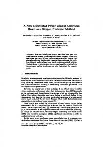
Seven-O’Clock: A New Distributed GVT Algorithm Using Network Atomic Operations David Bauer, Garrett Yaun, Christopher D. Carothers Murat Yuksel and Shivkumar Kalyanaraman Department of Computer Science Rensselaer Polytechnic Institute Troy, NY 12180, U.S.A. {bauerd,yaung,chrisc}@cs.rpi.edu, {yuksem,shivkuma}@ecse.rpi.edu 19th October 2005

Abstract

Global virtual time (GVT) algorithms must solve two key problems. The first is the transient message problem. Here, a message is delayed in the network and neither the sender nor the receiver consider that message in their respective GVT calculation. Thus, a GVT algorithm must account somehow for all messages scheduled. The second problem is called simultaneous reporting. This problem arises “because not all processors will report their local minimum at precisely the same instant in wall-clock time” [9]. Here, the underlying assumption is that event processing is allowed to continue asynchronously during the GVT computation which enables better overall parallel performance.

In this paper we introduce a new concept, network atomic operations (NAOs) to create a zero-cost consistent cut. Using NAOs, we define a wall-clock-time driven GVT algorithm called the seven o’clock algorithm that is an extension of Fujimoto’s shared memory GVT algorithm. Using this new GVT algorithm, we report good optimistic parallel performance on a cluster of state-of-the-art Itanium-II quad processor systems as well as a dated cluster of 40 dual Pentium III systems for both benchmark applications such as PHOLD and realworld applications such as a large-scale TCP/Internet model. In some cases, super-linear speedup is observed. We present a new measurement for determining the optimal performance achieved in a parallel and distributed simulation when the sequential case cannot be performed due to model size.

Asynchronous GVT algorithms rely on the ability to create a “cut” across the distributed simulation that divides events into two categories: past and future [9, 19]. GVT is then defined by the lower bound on unprocessed events in the “past” of the cut, which is in effect an estimate of the true GVT since events are being processed during its computations. Creating a cut can be done in several ways depending on the architecture of the machine(s) being used. For distributed computing platforms, the primary method of creating a “cut” is via message-passing as was defined by Mattern [19]. Here, messages are sent such that at most two cuts are made. The first cut signals the “start” of the GVT computation. The second cut, if needed based on message counts computed in the first cut, consider any transient messages discovered from the first cut. Please note, that these cuts need not be consistent. A consistent cut is defined as a cut where there is no message that was scheduled in the future of the sending processor but received in the past of the destination processor. These messages can be ignored because by definition they must be

The Seven O’clock algorithm greatly simplifies the GVT synchronization, which is unavoidable for traditional GVT algorithms by creating a zero-cost “consistent cut” across the distributed simulation.

1 Introduction At the heart of an optimistic parallel simulation system is the ability to reclaim memory from its virtual time past and re-use it to schedule future events as well as support state-saving operations as part of speculative event processing. Global virtual time (GVT) defines a lower bound on any unprocessed event in the system and defines the point beyond which events should not be reclaimed. Thus, it is imperative that the GVT computation operate as efficiently as possible. 1

Algorithm 1 Fujimoto’s Shared Memory GVT Algorithm: Variable Definitions.

Algorithm 2 Fujimoto’s Shared Memory GVT Algorithm: Initiate GVT

Global Variables int gvt_flag; lock_t gvt_lck; /* mutual exclusion variable */ int gvt_interval; /* number of time thru batch loop */ virtual_time_t lvt[npe]; /* LVT of each processor */ virtual_time_t gvt; Processor Private Variables virtual_time_t send_min_ts; /* account for events sent during GVT computation */ int status; /* current GVT state */

Steps to Initiate GVT within Scheduler Loop if(this processor is the MASTER) { gvt_cnt++; if( gvt_cnt >= gvt_interval AND processor status is GVT_NORMAL) { gvt_cnt = 0; if(gvt_flag == -npe) { lock(&gvt_lck); gvt_flag = npe; unlock(&gvt_lck); } set processor status to GVT_COMPUTE; }

scheduled at a time that is greater than GVT computed using a consistent cut. The “cuts”, while not consistent, effectively divide past from future in a causally consistent manner to solve the simultaneous reporting problem. Additionally, because of the use of message counts, it is able to determine if a second “cut” round is needed and traps any transient messages.

} else if (gvt_flag > 0 AND processor status is GVT_NORMAL) set processor status to GVT_COMPUTE;

In contrast, a shared memory multiprocessor greatly simplifies the GVT algorithm. Fujimoto’s GVT algorithm [8] generates a cut by setting a global flag positive. In a shared memory system this operation is observed on all processors in a causally correct order because the underlying hardware memory management mechanism ensures that no two processors will observe different orderings of memory references to a shared variable. Shared memory multiprocessor systems that adhere to this memory ordering model are called sequentially consistent [15]. The impact this memory model has on a GVT algorithm are that: (i) no messages are lost which prevents the transient message problem, and (b) the simultaneous reporting problem is solved because all processor effectively “observe” the start of the GVT calculation at the same instant of wall-clock time.

Algorithm 3 Fujimoto’s Shared Memory GVT Algorithm: Receive Events Steps to Receive Events and Anti-messages within Scheduler Loop move positive messages from shared memory message queue to processors priority queue. process any rollbacks. remove anti-messages from shared memory ‘‘cancel’’ queue. process any message cancellations and rollbacks.

2

Fujimotos GVT Algorithm and NAOs

We begin with an overview of Fujimoto’s GVT algorithm, as shown in Algorithms 1 – 5. Please note, there are minor modifications from the original algorithm presented in [8], but the correctness and efficient execution is preserved. These 5 parts are described as follows:

The motivation behind our research here is the question: Is there a method to achieve some of the benefits of sequentially consistent shared memory but in a loosely coordinated, cluster computing environment? The answer turns out to be yes. In this paper, we propose the idea of a network atomic operation (NAO), which enables a zero-cost cut mechanism which greatly simplifies GVT computations in a cluster computing environment. We demonstrate its reduced complexity by extending Fujimoto’s shared memory algorithm to operate across a cluster of shared-memory multiprocessors (SMP). We present a performance study using the PHOLD benchmark and TCP network model.

1. Variables (Algorithm 1): The key shared variable is the gvt_flag, which contains a mutual exclusion variable, gvt_lck. 2. Initiate GVT (Algorithm 2): The algorithm is initiated when the “master” processor iterates through the event scheduler loop gvt_interval times before set2

Algorithm 4 Fujimoto’s Shared Memory GVT Algorithm: Compute GVT

Algorithm 5 Fujimoto’s Shared Memory GVT Algorithm: Process and Schedule Events.

Steps to Compute GVT Once Initiated within Scheduler Loop

Steps to Process and Schedule Events within Scheduler Loop

if( processor status is GVT_COMPUTE ) { set processor status to GVT_WAIT lvt[my_pe] = min(send_min_ts, smallest event in priority queue); lock(&gvt_lck); gvt_flag--; if( gvt_flag == 0) { gvt = min( lvt[0] ... lvt[npe-1] ); gvt_flag = -1; set processor status to GVT_NORMAL; reset send_min_ts to max time value; unlock(&gvt_lck); collect processed events and state < GVT; if( gvt > end time of simulation ) goto DONE; } else { unlock(&gvt_lck); set processor status to GVT_WAIT; } } else if(processor status is GVT_WAIT AND gvt_flag < 0 ) { lock(&gvt_lck); gvt_flag--; unlock(&gvt_lck); if( gvt > end time of simulation ) goto DONE; collect processed events and state < GVT; set processor status to GVT_NORMAL; reset send_min_ts to max time value; }

Process smallest event in priority queue; if( sending a new event during event processing ) { enqueue message on destination receive queue; if( gvt_flag > 0 AND processor status is NOT GVT_WAIT ) send_min_ts = min( send_min_ts, time-stamp of new event); } DONE: compute parallel simulation stats and exit.

3. Receive Events (Algorithm 3): Here, new events and anti-messages are processed from arrival queues shared between processors. Each processor has its own externally exported, shared memory message queue that all other processors use to send events. A mutual exclusion lock is used around the queue to correctly serialize the arrival of either new events or anti-messages. Because of sequentially consistent memory, no message can be lost “in the network” and so the transient message problem is intrinsically solved. Observe that this “receive” and process rollbacks and anti-messages is a necessary step prior to computing any part of the GVT. It is also a normal step in every iteration through the scheduler loop. 4. Compute GVT (Algorithm 4): Once the new events and anti-messages are processed, each processor computes its local virtual time (LVT) value, which is the smallest unprocessed event that it is “aware” of, which includes any events it sent after the gvt_flag was set. This is denoted by send_min_ts. The last processor to compute its LVT also computes the minimum among all LVTs, which becomes the new GVT value. To inform other processors that the new GVT value is available, the gvt_flag is set to negative one. The last processor never “waits” for the GVT value and skips that state, while all other processors move to the “asynchronously waiting for GVT” state.

ting the gvt_flag equal to the number of processors (i.e., npe). Here is where the algorithm exploits the sequentially consistent memory properties. Every processor will “observe” the start of the GVT at the same instant in wall-clock time. More precisely, once the flag has been set, any other messages sent, are the responsibility of the sender, as shown in Algorithm 5. This provides a true separation between events in the logical past and logical future. When another processor observes the start of a GVT computation, it changes its status to “needs to compute an local virtual time (LVT)” This is denoted by send_min_ts.

5. Process Events (Algorithm 5): In this last step, forward event processing commences. Here, the smallest event is removed from the pending event set and processed. If 3

Algorithm 6 gvt_interval is a predefined number of iterations, and gvt_count is the current number of iterations. CPU 0: a. If(gvt_interval == gvt_count) b. set gvt_flag positive

Algorithm 7 Here, gvt_interval redefined as a measure of time usually in clock cycles, and not defined as the number of batch round through the scheduler. CPU 0: a. if(local clock time >= gvt_interval) b. start computing GVT

CPU 1: c. if(gvt_flag) d. start processing LVT

CPU 1: c. if(local clock time >= gvt_interval) d. start computing GVT

a new event is scheduled and the gvt_flag has been set greater than zero and the LVT value has not been reported (i.e., the processor should not be in the “wait” state), then it means this processor must consider this event in its LVT computation.

2.1

because most now provide a time-stamp counter, or clockcycle counter for performance measuring, such as the rdtsc instruction on all x86 series processors [12]. So we can compute wall-clock time based off of each processor’s time-stamp counter and synchronize these counters to a common view of wall clock time. Calls to reading the CPU clock adhere to the principles of a sequentially consistent memory model because wall clock time is consistent across all processors. Consider the following clock-based approach shown in Algorithm 7.

Network Atomic Operations

To directly extend Fujimoto’s GVT algorithm to a network of machines, would require a sequentially consistent distributed memory model, similar to what is provided in a shared memory system. As we described above, each processor observes the “start” of the GVT computation at the same wall clock time because of sequentially consistent memory. In reality, a processor attempting to read the flag may be stalled while the underlying system updates the local cache with the correct value of the flag. Consider the following abstracted view of the algorithm run in parallel on an SMP machine as shown in Algorithm 6. Running this code on a single processor defines the sequential consistency. The statements could be ordered on a single CPU as O = {a, b, c, d}. In this case both CPU 0 and 1 would begin computing GVT. However, if we change the interleaving of instructions to O = {a, c, b, d} then the GVT computation would only begin on CPU 0. CPU 1 would begin processing more events, but when an event is sent, the gvt_flag would be checked per the algorithm to ensure the sender correctly accounts for events during the GVT computation. The instruction, call it e, would then be accounted for by CPU 1 because e occurred after instruction b, and the consistent cut is properly formed. NAOs provide a similar functionality in a distributed system, however they are clock-based and not memory or statebased. The general concept is that an operation may occur atomically within a network of machines if all machines “observe” the event at the same instant of wall clock time. This functionality can be implemented on modern processors

If we again attempt to create a sequential ordering of instructions, it becomes obvious that any permutation is guaranteed to be consistent. Consistency is guaranteed because instructions a and c in Algorithm 7 will evaluate to true if and only if the same instance of wall clock time has passed for each CPU. Because we can only read the current wallclock time (as measured in clock cycles), any permutation of the possible orderings is valid because wall clock time is assumed to be same for all processors. There are limitations which we will discuss later in the paper. So NAOs may be characterized as a subset of the possible operations provided by a complete sequentially consistent memory model. For example, NAOs can only occur at predefined intervals, not dispersed throughout the timescale of the running application. Not only must NAOs occur at agreed upon intervals, but they must also take on a specific meaning or value. In the case of the GVT algorithm, we use NAOs to generate a consistent cut. The system is either in a GVT computation, or it is not. Further, GVT computations occur at a predefined frequency through the runtime of the application. An NAO cannot be used to give some global variable any value, because the only global variable in an NAO is wall clock time. However, any sequence of operations can be performed once the clock has been read. 4

2.2

Clock Synchronization

mine if a GVT computation has been started. There is no actual global variable, such as the gvt_flag in Algorithm 2, which signals the start of the GVT. Instead, we simply compute GVT every n units of wall-clock time. We have affectionately call this algorithm the “Seven O’clock Algorithm”. Seven O’clock comes from the idea that if we could have synchronized wall clocks on each network node, then we could simply compute GVT at well-defined intervals, i.e., every minute starting from seven o’clock, where seven o’clock is simply the start time of the scheduler. During the discussion of this algorithm we assume that each processor’s timestamp counter is perfectly synchronized with all of the other counters. We introduce the complexity of clock drift and jitter at the end. As we previously indicated, if one were to open up the underlying hardware implementation of a sequentially consistent shared memory system, a number of messages would be observed being passed over the memory bus between memory and cache modules. Also, any memory reads to a shared location could be blocked while waiting for the memory address to be made consistent. In particular, these consistency messages would either be well synchronized in time over a memory bus or acknowledged over a network depending on the architecture [10, 16]. Because we assume a distributed message passing system without acknowledgments, we need some additional information about the communications environment to avoid the transient message problem (i.e., events lost in the network). This problem can be overcome by adding a small amount of time to the NAO expiration, max_send_delta_t. Definition: max_send_delta_t is a worst case bound on the time to send an event through the network. This delta allows for the sending processor to account for remotely sent events which may cross the cut boundary. Note that this is not the same as delta causality which allows for excessively old events to be discarded. While it may seem unreasonable to assume such a value can be determined in practice, current cluster computing networks rely on high-speed switching fabrics. These fabrics typically have extremely low loss probabilities (1e − 12 or less) and can typically support the full bandwidth of all ports. Consequently, the worst case is experimentally computable and does not vary greatly from the average case. The states of the Seven O’Clock algorithm are shown in Figure 1 and are discussed below.

The heart of a network atomic operation is the assumption that all processors share a highly accurate, common view of wall-clock time. For this to occur, each processor’s timestamp or cycle-counter must be synchronized in some fashion. This is a well researched problem in distributed computing. The most recent, relevant result for our operating environment is by Ostrovsky and Patt-Shamir [21]. Here, the present provably optimal clock synchronization scheme where the clocks have drift and the message latency may be unbounded. Previous to this result, all other optimal results were based on non-drifting clocks. Moreover, they suggest that operational clock synchronization algorithms need not be general and “that they should work for the particular system in which they are deployed”. We take this view here. In particular, because of the time-scale of the clock is 1,000 times greater than message sends (i.e., nanoseconds vs. microseconds), clock drift rates can largely be ignored here. Additionally, since our contribution is not about clock synchronization algorithms, we used a simplified approach. To synchronize the clocks across all processors, we use a network barrier. Here, a master time keeper sends a synchronization message to each node, which responds back with its local time-stamp-counter. The master time keeper then sends a message to each processor with an appropriate time-stamp counter value that would be when in real-time measure in cycles the first GVT is to occur. Upon receipt of that message, each processor is released from the barrier and begins processing events. We recognize that for a large 1000 processor cluster, this approach has some scalability limitations. For such an operating environment, we would implement Ostrovsky and Patt-Samir algorithm [21]. Please note that this barrier synchronization occurs exactly once, during the initialization phase only. Re-synchronization of the clocks is unnecessary during the simulation because we are not running the experiments long enough to experience clock drift.

3

Seven O’Clock GVT Algorithm

We can now give a definition of a network atomic operation: Definition: An NAO is an agreed upon frequency in wallclock time at which some event is logically observed to have happened across a distributed system. Each processor in the system uses the NAO to determine the current state of the system depending upon the logical meaning of the NAO. For example, we use an NAO to deter-

• State A: Events are processed normally and not accounted for in GVT computation. This is no different 5

Figure 1: States of the Seven O’Clock Algorithm: from Fujimoto’s GVT Algorithm.

The only other differences between Fujimoto’s GVT algorithm and Seven-O’Clock are: (a) physically receiving messages and (b) physically sending messages. In the receiving step (Algorithm 3), all remotely sent new event messages and anti-messages are read from a communications channel, such as a socket. This is in addition to the shared memory queuing structures. From the standpoint of the GVT algorithm, it captures messages sent over either communications medium. Likewise, when a message is sent, the algorithm does not differentiate between which events are shared memory or offsystem messages.

• GVT “start”: The NAO signals the consistent start of the GVT to all processors, just as setting the gvt_flag in Fujimoto’s algorithm. • State B: Events sent during the max_send_delta_t interval are accounted for on the sending side. This is similar to how Fujimoto’s Algorithm uses gvt_flag to capture events the receiving processor might not consider in the sender’s LVT computation. Here, our algorithm reads the processor’s local cycle counter, determines if it is within the max_send_delta_t time of a GVT computation. If it is, then it captures this event’s timestamp against the minimum of any previously scheduled events during the max_send_delta_t time.

3.1 Proof of Correctness As previously noted, in order for a GVT algorithm to operate correctly, it must solve the transient message and simultaneous reporting problems. First, we assume all processors clocks are perfectly synchronized and there are no clock drift or jitter problems. We will relax this constraint later. Proof: To prove that a transient message cannot occur, assume that a transient message occurs in the scheduler. Then the time to send the event must be greater than the max_send_delta_t. But by definition max_send_delta_t is a worst-case bound on the time to send an event. This leads to a contradiction because the transient event took longer to send than the worst-case bound. Next, the simultaneous reporting problem occurs when all processors do not begin computing their local minimum at

• State C: Processors compute LVT by taking min(unprocessed events, events sent during B). This is identical to Fujimoto’s GVT Algorithm. • State D: Node 1 is first to complete local GVT algorithm and propagates this value to other nodes. • State E: Node 0 completes it’s local GVT algorithm and receives Node 1’s. It takes the minimum of the two and retransmits this value back to Node 1. The other processors check for the new GVT value at some point in the future and read the value from the shared memory. The processors return to state A. 6

message in epsilon time and not account for the event being sent. Consider the steps for remote sending of events: 1. Send the event. 2. Read local time-stamp clock. 3. If time_now + max_send_delta_t >= gvt_interval, then account for the event. Since epsilon is a value far less than max_send_delta_t, we must always account for the sent event. In the event that epsilon >= max_send_delta_t, we simply change our max_send_delta_t to have a larger value to overcome epsilon.

3.2

Problems with Clock-Based Algorithms

While the discussion of clock synchronization and its associated problems are outside of the scope of this paper, the Seven O’clock algorithm does provide a mechanism to solve each of these problems. Three problems arise in any clock-based algorithm: drift, jitter and synchronization error. During the course of a simulation, clocks may drift together, or apart. In the later case, this can lead to a gradual disparate view of time. Clock jitter occurs when a time is discretized and the width of the time units is not uniform. This can be a cause of clock drift over time depending on the frequency and size of the jitter. Finally, it is difficult to synchronize clocks to a high degree of granularity. This can lead to two processors being synchronized, but off by an indeterminate amount. Each of these problems can be dealt with in the Seven O’Clock algorithm by adjusting the definition of max_send_delta_t. Recall that this value is a worst-case bound on the time to send an event between two processors. We now redefine max_send_delta_t as the maximum of:

Figure 2: Simultaneous Reporting Problem: Source and destination processors see the cut being created at the same instant in wall clock time, so there is no opportunity for an event to “slip between the cracks”. the same instant. In fact, this is exactly what happens in the Seven O’clock algorithm. Because the consistent cut is generated using an NAO, each processor in the distributed system begins accounting for messages at precisely the same instant in wall clock time. Therefore this problem does not occur in this GVT algorithm as shown in Figure 2. Theorem: The simultaneous reporting problem cannot occur in a system where a consistent cut is defined across all processors at precisely the same instant in wall clock time. Proof: Assume to the contrary that the simultaneous reporting problem can occur. CASE 1: Assume each processor’s clock is perfectly synchronized with all other processor clocks. For the simultaneous reporting problem to occur, at least two processors must have different views of wall clock time. This is a contradiction because there only exists one notion of wall clock time. CASE 2: Each processor’s clock is synchronized with some degree of error, which is bounded by epsilon. In order for the problem to occur now, at least two processors must have different views of wall clock time, which differs by at most epsilon. This means that in epsilon time between two processors, a message was sent which was not accounted for. This is a contradiction because it is not possible to send a

1. worst-case bound on events sends 2. two times the synchronization error 3. two times the maximum clock drift during execution The max_send_delta_t parameter is simply an adjustment to the NAO to compensate for in-transit events that the sender must account for if they will not be received prior to the NAO expiring at the receiver. It can also be used to overcome the above mentioned problems when they are larger than 21 of the maximum send time. In Figure 3, two processors have drifted as far apart as is possible for a given run. As 7

ation cannot be aborted early because each network node is unaware of other nodes still actively processing events. The time wasted is bounded in the worst case by the size of the GVT interval. It is reasonable to expect this value to be small in relation to the overall time spent in execution, and so we do not consider this to be a major loss because it can be effectively amortized away. The fact we cannot force a GVT computation leads to the second limitation to the system. When all of the free events were consumed in the ROSS parallel scheduler, we were previously able to “jump” the GVT interval counter and force a GVT computation to occur. Refreshing the GVT value meant that we could reclaim at least one additional event in the system and continue forward processing. When free events are exhausted in the ROSS distributed scheduler we can no longer force GVT, and so must simply wait for the next GVT interval to pass. This problem occurs when we do not have sufficient optimistic memory to continue forward execution. The solution to this problem is to simply add more optimistic memory, or more network nodes, further distributing the model so that this does not occur. An indirect cause of this problem is speculative execution. In this case, stalled waiting for GVT to pass can act as a throttle on the faster nodes in the network such that they cannot overly speculatively execute, thereby creating the potential for long rollbacks. This problem is best solved by tuning the GVT interval to more closely match the amount of available memory. It is possible to force a GVT computation without disrupting the agreed upon NAO by simply sending a round of “force” messages. These messages would indicate that the NAO has pre-maturely expired and effectively changing the next NAO interval to immediate. Because we have not implemented this feature we cannot prove it’s correctness, however, we have not found it difficult to choose reasonable NAO settings. In the performance section of this paper we compute a design of experiments to determine the best setting for this variable.

Figure 3: Eliminating Clock Drift and Clock Synchronization Errors. The two processors are maximally misaligned. The remotely sent event cannot cross the cut boundary without being accounted for by the sender. long as max_send_delta_t is twice the maximum drift, it is possible for the sending processor to account for the event. In practice these values are several orders of magnitude smaller than the maximum time to send an event through the network, and can be safely ignored.

3.3

Limitations

Two issues arise from the introduction of the Seven O’clock algorithm that do not exist in other GVTs. Both stem from the general problem which is that the Seven O’clock GVT algorithm cannot be “forced”. First, GVT must advance for a simulation to determine that the simulation must end. In the Rensselaer’s Optimistic Simulation System( ROSS ) parallel scheduler this happens quickly because events to be scheduled past the end time are not processed and the GVT interval counter climbs quickly so that GVT may be computed when the system is effectively out of events. The Seven O’clock algorithm cannot be forced because each node must wait for the NAO to expire. At the end of a simulation, the ROSS system has no events scheduled for processing, and is simply waiting for the CPU to compute the next GVT interval. This situ-

3.4 Uniqueness The Seven O’clock GVT algorithm is unique because it uses synchronized Real-Time Clocks as the global invariant. No message passing is required to communicate the current view of time among the processors. While algorithms such as Mattern’s or Samadi’s can be made scalable, there is no lower cost than reading the timestamp counter on a CPU for constructing a consistent cut. This fact leads us to believe that the Seven 8

Cut Calculation Cost Parallel/Distributed Global Invariant Independent of Event Memory

Fujimoto O(1) P Shared Memory Flag N

7 O’clock O(1) P+D Real Time Clock Y

Mattern O(N) or O(log N) P+D Message Passing N

Samadi O(N) or O(log N) P+D Message Passing N

Table 1: Comparison of major GVT algorithms to Seven O’clock. r-PHOLD: 1,000,000 LPS, 10% remote, 16 start events

O’clock algorithm must be the most efficient cut algorithm possible. This is equivalent to the cost of Fujimoto’s algorithm for shared memory processors. It is difficult to imagine a smaller cost cut algorithm that the setting of a global variable. Table 1 compares the Seven O’clock algorithm to other widely known algorithms. The most important difference with the Seven O’clock algorithm is that it is the only known algorithm which is entirely independent of the available event memory. Seven O’clock relies on a real-time clock frequency that allows us to begin to view event processing in terms of the frequency domain rather than the spatial domain. Each of the other GVT algorithms execute GV T interval ∗ Batch events between GVT epochs. In our algorithm, we are allowed N AOInterval time between GVT epochs, and so the number of events processed is indeterminate based on the interval frequency and speed of the individual CPU(s). While outside the scope of this paper, performing a spectral analysis is useful in determining the power of a given model. Spectral analysis may also lead to automatic filtering and compression of model spaces when computing design of experiments.

4

1.8e+06 Optimal 1 node 2 node 3 node 4 node

1.6e+06 1.4e+06

Event Rate

1.2e+06 1e+06 800000 600000 400000 200000 0 2

4

6

8

10

12

14

16

Number of Processors

Figure 4: PHOLD results in the distributed cases with 1,2 or 3 processors utilized per node. The 4 processor cases are clearly affected by context-switching in the operating system for I/O operations.

uted random number generator in the range of 0 to 100. If the generated value is less than the specified percent of remote messages allowed, we choose the destination LP over an exponential distribution of all LPs, otherwise, the event will be sent to the source LP. The third call determines the offset timestamp for events and is exponentially distributed with a mean of 1.0, with the model completing at timestamp 100. For all experiment runs, we mapped LPs to Processing Elements (PE) in a round robin fashion. Each simulation run contained 1 million LPs, and the number of Kernel Processes 2 (KP) was determined as Ncpu ∗ multiplier. The multiplier was experimentally determined, as is explained in the next section. The message population per LP is 16. This model is a pathological benchmark which has minimal event granularity while producing a configurable number of remote events which can result in “thrashing” rollbacks. In [3], KPs where introduced as an aggregation structure for reducing LP fossil collection and rollback. One modification to this model

Performance Study

There are two benchmark models used in this performance study. The first is a synthetic workload model called PHOLD. This commonly used benchmark has been modified to support reverse-computation and is configured to have minimal Logical Process (LP) state, message sizes and event processing. The forward computation of events involves computing three random numbers: one for computing if a remote event should be created, one used to compute the time-stamp and one used for the destination LP. The reverse computation involves “un-doing” an LP’s random number generator (RNG) in order to restore it’s state. Because the RNG is perfectly reversible, the reverse computation restores seed state by computing the perfect inverse function as described in [3]. The destination LP is determined by calling a uniformly distrib9

was the ability to constrain the number of remote events created by the LPs. This allows us to analyze the system under varying workloads. The overhead The second application is a model of TCP and this implementation follows the Tahoe specification [6]. There are three main data structures in this model: the data packet which is sent between hosts in the forwarding plane, the network router LPs which maintain queuing information and forward packets through the network and the host LPs which keep statistical information on the transferring of data. For detailed model design and implemented, we refer the interested reader to [26]. For all TCP experiments we use the campus network defined in [29] which has been widely used to benchmark many network simulations in the past. We create a large-scale topology from this small network in the same approach used by Perumulla in [30], that connects multiple campus networks together to form a ring.

mine how major facilities such as the GVT computation and fossil collection are performed. For example, most GVT algorithms define GV T Interval batch loops be performed between successive GVT computations. Determining the best values for any simulator is difficult because every model is different and it is difficult to know which settings yield the best performance for a given model. Even within a single execution of a given model the performance of the model may change. For example, in the TCP model we present here, the TCP LPs which originate the data in the network have a much higher event granularity than do the internal IP routers which simply forward data traffic events through the network. The Seven O’clock algorithm increases this complexity because the time between GVT computations is not based on the number of events processed, but on the N AOInterval alone. This means that between any two GVT computations a variable number of events will be processed. Design of Experiments or “experiment design” is a well known branch of performance analysis, specifically, a sub branch of statistics [44, 45]. It has been used extensively in areas such as agriculture, industrial process design and quality control [45] , and has been introduced to the area of practical computer and network systems design by Jain [44]. Statistical experiment design views the system-under-test as a black-box that transforms input parameters to output metrics. The goal of experiment design is to maximally characterize (i.e. obtain maximum information about) the black-box with the minimum number of experiments. Another goal is robust characterization, i.e., one that is minimally affected by external sources of variability and uncontrollable parameters, and can be specified at a level of confidence.

4.1 Computing Testbed and Experiment Setup Initial results were collected on 4 quad-processor Itanium servers. The Itanium-2 processor [11] is a 64 bit architecture based on Explicitly Parallel Computing (EPIC) which intelligently bundles instructions together that are free of data, branch or control hazards. This approach enables up to 48 instructions to be in flight at any point in time. Current implementations employ a 6-wide, 8-stage deep pipeline. A single system can physically address up to 250 bytes and has a full 64-bit virtual address capability. The L-3 cache comes in a 3 MBs configuration and can be accessed at 48 GBs/second which is the core bus speed. TCP over Gigabit Ethernet was used as the interconnection network. The Netfinity cluster at RPI is a Red Hat Linux 9.0 cluster consisting of 40 machines, for a total of 80 processors. Each machines is a Symmetric Multi-Processor (SMP) machine with two 800MHz Pentium III processors. The 2 CPUs of each machine share 512 MB of RAM. The 40 SMP machines are connected to each other via a gigabit ethernet switch. The Sith cluster computing platform at Georgia Tech is a Linux cluster consisting of 30 machines, for a total of 60 CPUs. Each machine is a Symmetric Multi-Processor (SMP) machine with two 900MHz Itanium processors. The 2 CPUs of each machine share 4 GB of RAM. The 30 SMP machines are connected to each other via a gigabit ethernet switch with EtherChannel aggregation. All simulators have several input parameters which deter-

In order to determine the settings that will yield the best for the PHOLD model, we use the Unified Search Framework (USF) [35] and the heuristic algorithm Random Recursive Search [34]. By using Recursive Random Search (RRS) approach to design of experiments, we find: (i) that the number of simulation experiments that must be run is reduced by an order of magnitude when compared to fullfactorial design approach, (ii) it allowed the elimination of unnecessary parameters, and (iii) it enabled the rapid understanding of key parameter interactions. From this design of experiment approach, we were able to experimentally determine the settings which yielded the highest performance for the PHOLD model in a relatively small number of experiments. The best parameter settings for the TCP model were determined ad-hoc because of time limitations. 10

NumCPU Voluntary CS 2 3 4

Involuntary CS 0 0 46

Total CS 12 14 1123

may lead to confusion [39] or even abused depending on how they are used [40, 42, 43]. Our interest in introducing a new measurement is two-fold. We would certainly like to be open and honest about our performance results, and eliminate any possible sources confusion. Second, we would like to be able to easily compare against previous work.

Table 2: PHOLD context switching in the OS degrades performance when the simulation “conflicts” with other system processes.

In performing large-scale simulation it is not always possible to generate a sequential case for speedup comparison. One constraint of Amdahl’s law is that the same instructions be processed for the sequential case, as are processed during the parallel case. One approach to overcome this problem is to use the results from the smallest configuration possible as the basis for the sequential time. This is problematic because, while this minimizes the costs of parallelization, it does not reduce them entirely, leading to an under-estimation of optimal performance. The benefit of this approach however, is that the model being measured is exactly the model used to generate the sequential time.

Optimistic event memory was computed in each case from the following formula: OptimisticM emory = ceil(g_tw_nlp/g_tw_npe) ∗ phold_start_events ∗ multiplier where multiplier was fixed at 2. Here, g_tw_npe is the number of processors used within the cluster configuration, and g_tw_nlp is the total number of LPs. During distributed execution, each processor can consume approximately N AOT ime/AvgT imeT oComputeOneEvent per GVT epoch.

In [30], the extrapolation was to generate a smaller model running on a single machine from the largest execution, and to “grow” those results up to the full model size. This approach leads to an over-estimation of the optimal because the model used to generate the sequential case is not the actual model being measured. While this is a highly accepted scientific method used for determining performance improvements, we show here how the physical nature of the hardware can fluctuate from those results, creating anomalies which are unexplainable by this method. These anomalies can only be explained by taking the actual model being measured into account when computing the sequential case. We note that while this approach was appropriate for the model in [30], it does not work in the general case.

4.2 PHOLD Performance Data 4.2.1

Measuring Performance

In [5], we configured PHOLD with 10% remote messages, 16 seed events per LP and used the Myrinet network. Figure 4 illustrates super-linear results on a small cluster of 4 Itanium-II machines. Comparing the results in the parallel and distributed case is complicated because we have results based both on the number of processors used and based on the number of nodes used. We start by considering two nodes maximizing the processors before increasing the number of nodes. Then we consider three nodes, and finally four nodes. Performance begins to degrade once a configuration becomes overly parallelized. In each node case, when we added the final processor per node, performance degraded due to context switching in the operating system for I/O operations. We informally measured the amount of context switches which occurred in each case and found that the four processor case typically generated greater than 100 times the number of context switches, as shown in Table 2. Measuring speedup is an attempt to determine the cost of synchronization in a parallel and distributed environment. Typically Amdahl’s law [38] and Gustafson’s law [41] are applied by first performing the sequential simulation of the model, and then comparing each subsequent parallel execution to that. An examination of these laws is outside of the scope of this paper, but it is widely accepted that this laws

Clearly a more precise approach is needed for measuring the performance of parallel and distributed systems. A new approach should take into account all of the particular details of the underlying hardware, and provide an optimal solution which cannot be superseded by a super-linear result. Besides context switching, other problems may arise such as memory bus overloading or serialized memory references [2, 16, 20], which limit the possible speedup due to parallelism. By maximizing the number of nodes used in a simulation it is possible to avoid or reduce these problems by de-coupling the hardware systems which are limiting performance, and this too must be taken into account when determining the optimal performance characteristics for a given model. In the following sections we outline a general approach for 11

15 CPU, 15 Nodes, 10% Remote

Performance: 1 Million LPs, 16 Start Events Per LP

1.27e+06

5.5e+06 10% CalQ Linear Perf 10% Actual Perf 25% Actual Perf

5e+06 1.26e+06 4.5e+06

Event Rate (events / second)

Events Per Second

1.25e+06

1.24e+06

1.23e+06

1.22e+06

1.21e+06

4e+06 3.5e+06 3e+06 2.5e+06 2e+06 1.5e+06 1e+06

1.2e+06 500000 1.19e+06

0 0

10

20

30

40

50

60

70

80

90

100

10

Experiment Number

Min 16 0.01 450

Max 4096 0.50 9000

24

28

32

36

Figure 6: Results for 10% and 25% remote messages using increasingly more Netfinity nodes. Linear speedup for the 25% remote model was nearly identical.

Step 32 0.01 2

the variance on the input parameters. These input parameters were chosen because of their effect on the major simulator facilities, including GVT, event processing and fossil collection. The input parameter for the number of KPs is actually a multiplier and the number of KPs was selected as 2 Ncpu ∗ KP _M ultiplier.

Table 3: Input parameters to simulator used in design of experiments

Selecting from the best input parameter settings, a full node configuration was computed using the Netfinity cluster. The best settings for 10% remote events were a batch size of 2531, and NAO of 0.36 seconds and a KP multiplier of 2. The best settings for 25% remote events were a batch size of 886, an NAO of 0.24 seconds and a KP multiplier of 12. The 25% model response was also approximately 5%. Results shown in Figure 6 indicate excellent linear performance for 10 and 25% remote events. Super-linear performance was achieved on the Itanium cluster primarily because of the highly optimized memory hardware and because we were able to generate a “true” sequential execution time. Linear performance on the Netfinity cluster was determined by using the LP mapping for the 36 node, 10% remote event, case, and extrapolating what the sequential case would have been. This is an accepted scientifically accepted approach for calculating linear performance speedup, but it should be noted that this approach over-states the potential speedup possible because the model used for the sequential case is not the same model being measured.

measuring the optimal performance of a parallel and distributed simulation that considers not only the hardware used but also the model used, and the LP mapping of that model to the underlying hardware. 4.2.2

18

Number of Processors

Figure 5: Simulator variation measured by design of experiments using Random Recursive Search. Parameter Batch Loop Size NAO Interval (seconds) Number of KPs

14

Experiment Design

With several input parameters which affect the raw performance of the simulation, it is necessary to compute a design of experiments to quantitatively categorize the system under test. For this purpose, we utilized the Unified Search Framework (USF) [35] to create a design of experiments. Because we are only interested in the highest degree of performance, we used the Random Recursive Search algorithm [34] within USF to quickly determine the best settings for a particular configuration of the PHOLD model. The need for a design of experiments is illustrated in Figure 5. There is a variation of approximately 5% from the best to the worst experiment, varying the input parameters: NAO interval, size of the batch loop, and the number of KPs used. Table 3 shows 12

4.2.3

Measuring Optimal Performance: Distributed

Performance: 1 Million LPs, 16 Start Events Per LP 9e+06

Computing the sequential case for performance comparison is not always possible for large-scale models. The purpose of computing the model sequentially is to determine the optimal performance without overhead due to parallelization. In this section we outline a novel approach for determining the optimal performance of the simulator software given a specific model, hardware configuration and model LP mapping to the hardware. Whenever we make improvements to simulator engine facilities, we are attempting to improve performance. At some point, there must exist an achievable optimal performance beyond which further improvements to the software would not be able to generate additional speedup. In the past others have determined a sequential case by running large-scale models on the minimum hardware required. But this approach understates the optimal case because it contains code necessary for resolving contention and communication issues. In addition, this approach also leads to super linear performance when enough CPU L2 caches are added to the configuration. Super linear performance occurs because as more compute nodes are added to the hardware configuration, more of the model will fit into the L2 cache, and a speedup is gained by the nature of the hardware. Another problem in determining a base case for performance is in the mapping of the model to simulator entities (PEs or KPs). Radically different performance can be measured within the same model when LPs are mapped differently to PEs because the mapping largely determines the communication and contention load in the system. To overcome these problems, we asked ourselves if there was a way in which we could generate a sequential case over all of the CPUs used per simulation run. In fact, we wanted to be able to run one instance of the sequential scheduler within ROSS per CPU. In order to do this however, LPs could no longer send events to LPs scheduled on remote CPUs. In order to implement this approach, it was necessary for us to be able to modify the models in such a way that this did not occur. Using this approach we were able to take into consideration the hardware configuration, and the specific model and its mapping of LPs to the hardware. To determine the optimal performance for the Netfinity cluster, we simply re-compute the PHOLD model, but this time each event’s destination LP is always the sending LP. When we constrain the model in this way we no longer require the parallel scheduler, since we know there will be no

Optimal Perf 10% Actual Perf 10% Linear Perf

8e+06

Event Rate (events / second)

7e+06

6e+06

5e+06

4e+06

3e+06

2e+06

1e+06 10

14

18

24

28

32

36

Number of Processors

Figure 7: Results for PHOLD configured with 10% remote events, compared to the Optimal Performance possible for the available hardware. The linear performance curve remains for comparison.

contention issues. So, we replace the parallel scheduler with the sequential scheduler and re-execute the model for the desired node configurations. It is important to note that by using the sequential scheduler, we eliminate simulator facilities such as the GVT computation and fossil collection. Also, because each event is now sent in “loopback” mode, the network connecting the nodes is not utilized during the simulation. A key observation is that the model continues to commit the same instructions and events that will be committed during normal execution. For example, even though each event in the optimal case is sent in loopback mode, we continue to compute the destination LP. This means that we continue to execute the same lines of code as in the model being measured. Comparing the PHOLD model used to determine the optimal performance to the PHOLD model measured, there was a difference of approximately 3,000 events out of over 161 million events computed. This represents about 2.2e-5% of variance, but more importantly, the amount of work computed by the model can be considered equal. Figure 7 shows the actual results plotted against both the Linear Speedup curve as well as the new Optimal Performance curve. This is done to illustrate the difference between the two measurements. This figure illustrates the problem with computing speedup in the typical way. Clearly the linear performance over-states the actual performance gained 13

the underlying hardware or network used, then it must be the model which is causing the performance anomaly. In addition, we can rule out major simulator facilities such as GVT or fossil collection as the cause because they do not exist in the optimal performance curve. The LP mapping must be the cause for these irregularities because it is the only constant for both curves which could account for the observed behavior. This is an important distinction because this clearly illustrates not only what the optimal performance should be for the given model and hardware, but also given the way in which the model is mapped for parallelization. Figure 8 shows that PHOLD with 25% remote messages contain the same anomaly, because we have maintained the LP mapping. In order to clearly (and honestly) represent performance results, it is necessary to plot the optimal or linear curves to produce a proper scaling. The results in Figure 8 do not illustrate good linear improvement. The improvement for 36 nodes is only 2 times that of 10 nodes. We address this special case in the subsequent section. Clearly one limitation to this approach is that it may not be possible to generate the same critical path workload distributed across multiple sequential schedulers for every model. However, if we want to determine as honestly as possible the speedup achieved by improvements within the software via either engine improvements or LP mappings, it is clear that this approach is viable when possible.

Performance: 1 Million LPs, 16 Start Events Per LP 1.2e+06 25% Actual Perf 1.1e+06

Event Rate (events / second)

1e+06

900000

800000

700000

600000

500000

400000 10

14

18

24

28

32

36

Number of Processors

Figure 8: We see the same effects of the LP mapping in the 25% remote event PHOLD model. (The optimal performance curve is not shown due to scaling.)

because it could not take into consideration this model’s LP mapping and the hardware used. We believe that our approach to measuring performance for large-scale models more clearly illustrates the performance of the simulation executive software because it takes into account not only the model, but also the underlying hardware limitations. For example, as the number of nodes used increases, the model should perform increasingly better because more and more of the model fits into the L2 caches. The optimal performance measurement accounts for this behavior, while the linear speedup curve does not. To properly use the old measurement also requires computing the sequential case for each cluster configuration, otherwise the performance for the smaller configurations will be under-stated. The optimal performance measurement is correct for each cluster configuration and is therefore a more realistic measurement of the model for the given hardware and mapping. Most importantly, the optimal performance measurement is only theoretically achievable and super-linear results beyond this are unlikely because even if overhead due to parallelization were eliminated entirely, you would be left with the optimal case.

4.2.4

Optimal Performance: Parallel and Distributed

In [5] we observed a performance drop whenever the last CPU on a cluster node was mapped for the simulation. We have identified the cause of this behavior to be a high overhead due to context switching within the OS for I/O operations. In order to quantify the amount of loss due to context switching requires that we look at the speedup available in parallelization alone. Figure 9 shows both the linear speedup and optimal performance achievable on a single Netfinity cluster node. This illustrates that linear speedup is not achievable through software alone on this hardware. This is likely due to limitations on the memory bus between the two processors, as we have measured in the past [3]. It is helpful to know what speedup the hardware will allow when measuring the performance of the simulator software. Taking the hardware into consideration, ROSS performs within 25% of the optimal performance achievable through software alone. Figure 10 shows the distributed and parallel

The performance curves illustrated in Figure 7 clearly dip slightly around 14 nodes used, and again at 32 nodes. We changed the machines used to collect these results several times and found that the curves overlapped with less than 0.1% variation. If the performance is not dropping due to 14

Parallel Speedup: 100,000 LPs, 16 Start Events Per LP 500000 Optimal Perf Linear Speedup 10% Remote 450000

Event Rate

400000

350000

300000

250000

200000 2

1 Number of Processors

Figure 9: For 100,000 LPs, ROSS’ parallel scheduler generates a speedup of 1.4. However, when we compare to the measure of optimal performance, we see that we are within 25% of optimal.

Figure 11: Campus Network [29] In this section we have shown how measuring linear performance is imprecise for large-scale distributed simulation because it is difficult if not impossible to maintain the hardware restrictions for fair comparison or to compute the costs of associated with the hardware. We have proposed a new measurement called Optimal Performance, and shown how to collect the result. Optimal performance measures exactly how fast the given hardware can execute events for a given model. This new measurement formalizes the performance level of the actual simulator performance, regardless of model size or LP mapping. Intuitively, simulator performance should not exceed the optimal case. We believe that this measurement will greatly simplify performance analysis of parallel and distributed simulation.

2 CPU per Node, 1 Million LPs, 16 Start Events Per LP 2.4e+06 10% Remote Events 25% Remote Events 2.2e+06 2e+06

Event Rate

1.8e+06 1.6e+06 1.4e+06 1.2e+06 1e+06 800000 600000 400000 20

30

40

50

60

70

4.3 TCP Performance Data

80

Number of Processors

4.3.1

Figure 10: Results for PHOLD on the Netfinity cluster. A speedup of approximately 2 is achieved from 20 to 72 processors.

TCP Model Comparison

Figure 11 illustrates the campus network, widely used to benchmark many network simulators [30, 31, 36, 33, 32] and is an interesting topology for network experimentation [37]. The campus network is comprised of 4 TCP servers, 30 routers in 4 LANs, and 504 TCP clients for a total of 538 nodes [29]. Limitations in our TCP model caused us to have 504 HTTP servers, one to serve each client. In addition, in order to maintain proper queue statistics at the client links, it was necessary to add an aggregation router per 10 or 12

results remain far below this level for 2 CPU per node configurations. The primary reason for the poor performance on the Netfinity cluster is the context switching overhead introduced to handle the network I/O operations, and not attributable to ROSS. Figure 4 does not indicate the same slowdown until we add the fourth and final processor to the configuration. 15

Distributed ROSS: TCP-Tahoe Model 1e+07 1 CPU per Node 2 CPU per Node Linear Performance

9e+06 8e+06

Event Rate

7e+06 6e+06 5e+06 4e+06 3e+06 2e+06 1e+06 0

Figure 12: Ring of 10 Campus Networks. [30]

4

8

1618

24 28

36

48

56

72

Number of Processors

Figure 13: TCP model performance improves linearly, exhibiting a super-linear speedup. Comparing to the optimal performance leads to a higher quality analysis of simulator performance.

client nodes. Our equivalent campus resulted in 1082 node LPs. Because the networks are equivalent, we refer to our campus network model as having 538 nodes for ease of comparison. The campus network is comprised of 4 different networks. Network 0 consists of 3 routers, where node zero is the gateway router for the campus network. Network 1 is composed of 2 routers and the servers. Network 2 comprised of 7 routers, 7 LAN routers, and 294 clients. Network 3 contains 4 routers, 5 LAN routers, and 210 clients [30]. All router links have a bandwidth of 2Gb/s and have a propagation delay of 5ms with the exception of the network 0 to network 1 links, which have a delay of 1ms. The clients are connected to their LAN router with links of bandwidth 100Mb/s and 1ms delay.

Nodes Used 2 4 8 16 32

ROSS 341853 730720 1493702 2817954 5508404

PDNS n/a n/a n/a in swap 1069905

Table 4: Performance results measured for ROSS and PDNS for a ring of 256 campus networks. Only one processor was used on each computing node. Rates are packets executed per second.

For our experiments we connected multiple campus networks together at their gateway routers to form a ring. The links connecting the campuses together were 2Gb/s with delays of 200ms. Figure 12 shows a ring of 10 of these campuses connected. The traffic was comprised of TCP clients in one domain connecting to the server in the next domain in the ring. The server would transfer 500,000 bytes back to the client application. This approach replicates the network created for PDNS by Kalyan Permulla for [30]. We connected 1,008 campus networks together to create a network of size 542,304.

We attempted to reproduce a model of similar size in PDNS on our Netfinity cluster but the memory requirements where too high for only 40 machines. The largest PDNS model that we could get to run was 137,728 LPs using 32 cluster nodes. We were able to execute this model on one node in ROSS and the results and performance numbers can be seem in Table 4. ROSS was able to achieve 5.5 million packets per second whereas PDNS processed 1.07 million packets per second. This shows that our ROSS implementation has a significantly smaller memory footprint and achieves 5.14 times in speedup over PDNS.

Figure 13 shows a super-linear speedup on the one processor case per node. This can be attributed to the decrease in context switching from the two processor per node case. This is a similar result to what was observed in the PHOLD results presented in [5]. 16

TCP Performance: 1 CPU per Node

TCP Performance: 2 CPU per Node

6e+06

1.2e+07 Optimal Perf Actual Perf

Optimal Perf Actual Perf 1.1e+07 1e+07 Event Rate (Events per Second)

Event Rate (Events per Second)

5.5e+06

5e+06

4.5e+06

4e+06

9e+06 8e+06 7e+06 6e+06 5e+06 4e+06 3e+06

3.5e+06

2e+06 16

18

24

28

16

Number of Processors

36

56

Number of Processors

Figure 14: TCP model performance improves linearly. Optimal performance achieves a speedup of about 1.6, and the actual performance about 1.35.

Figure 15: TCP model performance improves linearly. Optimal performance achieves a speedup of about 3.3, and the actual performance about 2.5.

4.3.2 Optimal Performance

from “slipping through the cracks” [9]. In addition to Fujimoto’s and Mattern’s GVT algorithms, there have been a number of predecessors. Preiss [23] introduced a scheme which places the PEs into a ring. The first round completes when a token has been passed around the ring and returns to the initiating PE. When the initial token is received, a PE begins accounting for remotely sent messages which may or may not complete prior to the GVT computation. On receiving the second token, a local GVT value is computed as the minimum between the value stored in the token and the PEs local minimum. Improvements to this algorithm have been proposed by Bellenot [1] which reduce the complexity of message passing by organizing PEs into trees rather than a ring. Lin and Lazowska [17] propose a new data structure that reduces the frequency of acknowledgment messages. The work done by Tomlinson and Garg [24] uses counters to detect transient messages. However, this scheme does not employ the use of a “cut” as Mattern’s algorithm does. Pancerella [22] propose a hardware based scheme whereby host systems using custom network interface cards are interconnected to form an efficient reduction network to rapidly compute GVT.

In order to measure the optimal performance of the TCP model, we connected each TCP client to a server within the local campus, rather than a remote campus within the ring. This allowed us to run the TCP model in the expected configuration without changing the execution or mapping of the model. We measured the TCP model’s optimal performance using the Sith Itanium cluster at Georgia Tech. Comparing TCP performance to optimal performance indicates that ROSS performance is not in fact super-linear when the hardware and model mapping is taken into account. Figure 14 shows that the actual TCP model performance achieves a speedup of approximately 1.35, compared to a possibly 1.6 in optimal performance. Similarly, Figure 15 shows that for two CPUs utilized per node, the TCP model achieves a speedup of 2.5 compared to a possible 3.3 optimal.

5 Related Work Samadi’s algorithm [25] solves the simultaneous reporting problem through the use of message acknowledgments. Here, processors will tag any “ack” message that it sends in the period from when the processor reports its LVT until it receives the new GVT value. This process prevents any messages

In follow-up research, Lin [18] uses control messages to efficiently find/flush out transient messages. At about the same time, D’Souza et. al [4], proposes a statistical approach to estimating GVT. 17

References

Prior to Fujimoto’s GVT algorithm, Xiao et al. [27], proposes an asynchronous GVT algorithm that exploits sharedmemory multiprocessor architectures. Here the concept of “cages” is used, where each processor own some set of “cages” that it places or lays down in order to track the LVT of that processor. It is interesting to note, that here a global Cage Flag much like the gvt_flag in Fujimoto’s Algorithm, is used to “kick off” the GVT computation.

[1] S. Bellenot, “Global Virtual Time Algorithms”, In Proceedings of the SCS Multiconference on Distributed Simulation, Vol. 22, pp. 122–127, 1990. [2] C. D. Carothers, K. S. Perumalla, and R. M. Fujimoto, “The effect of state-saving in optimistic simulation on a cache-coherent non-uniform memory access architecture,” in Proceedings of the 1999 Winter Simulation Conference, 1999.

Related to both “consistent cuts” and sequentially consistent memory is the issue of causality. Most recently, Zhou et al [28], propose a “relaxed” causal receive ordering algorithm called critical causality for distributed virtual environments.

6

[3] C. D. Carothers, D. Bauer, and S. Pearce, “Ross: A high-performance, low memory, modular time warp system,” Journal of Parallel and Distributed Computing, 2002.

Conclusions and Future Work

[4] L. M. D’Souza, X. Fan, and P. A. Wilsey, “pGVT: An Algorithm for Accurate GVT Estimation”, In Proceedings of the 8th Workshop on Parallel and Distributed Simulation (PADS ’94), pp. 102–109, 1994.

We present a new idea, Network Atomic Operations, and apply it to solving the global virtual time problem. We use an NAO to generate a zero-cost cut in a distributed system which is both scalable and efficient. We also propose a new approach to measuring optimal performance for parallel and distributed simulation. This approach eliminates super-linear results from being reported by taking into account the underlying hardware, as well as the model and the model mapping for parallelization.

[5] D. Bauer, G. Yaun, C.D. Carothers, M. Yuksel, and S. Kalyanaraman, “Seven-O’Clock: A New Distributed GVT Algorithm Using Network Atomic Operations”, In Proceedings of the Workshop on Parallel and Distributed Simulation (PADS ’05), 2005. [6] K. Fall and S. Floyd, “Simulation-based comparison of tahoe, reno, and sack tcp,” Computer Communication Review, vol. 26, pp. 5–21, 1996.

Network Atomic Operations allow us to view the behavior of Time Warp in the frequency domain because they define the relationship between virtual time and wall-clock time. In the future, we would like to investigate maximum rollback lengths using NAOs. Computing a spectral analysis of the Time Warp system should allow us to analyze the system and detect when the forward processing of events is optimal. These results should allow us to place a bound on the maximum rollback distance possible for a given model configuration. If we know the maximum rollback distance, it may become possible to eliminate the GVT computation completely.

[7] R. M. Fujimoto, “Time warp on a shared memory multiprocessor,” in Proceedings of the 1989 International Conference on Parallel Processing, vol. 3, pp. 242–249, August 1989. [8] R. M. Fujimoto and M. Hybinette, “Computing global virtual time in shared-memory multiprocessors,” ACM Trans. Model. Comput. Simul., vol. 7, no. 4, pp. 425– 446, 1997.

In addition we have proposed a new performance metric for simplifying the analysis of parallel and distributed simulator performance. In the future we hope to discuss the percentage of optimal achieved by a given simulator. It would be interesting to investigate if that percentage holds for varying cluster architectures and configurations. Our assumption is that it would not and that certain simulators would see better performance on certain architectures.

[9] R. M. Fujimoto, Parallel and Distributed Simulation Systems. "John Wiley and Sons, Inc.", 2000. [10] K. Garachorloo et al. “Memory Consistency and Event Ordering in Scalable Shared-Memory Multiprocessors”, Proceedings of the 17th Annual Symposium on Computer Architecture, pp. 15–26, 1988. 18

[11] Intel, “Intel Itanium-II Reference Manuals”, Available via the web at: http://www.intel.com/ design/itanium/documentation.htm?iid= ipp_srvr_proc_itanium2+techdocs&

Parallel Discrete-Event Simulation”, In Proceedings of the 7th Workshop on Parallel and Distributed Simulation (PADS ’93), pp. 52–59, 1993. [23] B. R. Preiss, “The Yaddes Distributed Discrete Event Simulation Specification Language and Execution Environments”, In Proceedings of the SCS Multiconference on Distributed Simulation, vol. 21, March, pp. 139–144, 1989.

[12] Intel, “Intel Pentium 4 and Xeon Processor Optimization Reference Manual,” Available via the web at: http://developer.intel.com/design/ pentium4/manuals/248966.htm [13] D. Jefferson, “Virtual Time”, ACM Trans. Prog. Lang. and Systems, vol. 7, no. 3, July, pp. 404–425, 1985.

[24] A. Tomlinson and V. K. Gang, “An Algorithm for Minimally Latent Global Virtual Time”, In Proceedings of the 7th Workshop on Parallel and Distributed Simulation (PADS ’93), pp. 35–42, 1993.

[14] D. Jefferson, “Virtual Time II: Storage Management in Distributed Simulation”, In Proceedings of the 9th Annual ACM Symposium on Principles of Distributed Computing, August, pp. 75–89, 1990.

[25] B. Samadi. “Distributed Simulation, Algorithms and Performance Analysis”, Ph. D. Thesis, University of California, Los Angeles (UCLA), 1985.

[15] L. Lamport, “How to Make a Multiprocessor Compute that Correctly Executes Multiprocess Programs”, IEEE Transactions on Computers, vol. 28, no. 9, September, pp. 690–691, 1979.

[26] G. Yaun, C. D. Carothers, and S. Kalyanaraman, “Large-scale TCP models using optimistic parallel simulation,” In Proceedings of Workshop on Parallel and Distributed Simulation (PADS 2003), June 2003.

[16] J. Laudon and D. Lenoski, “The sgi origin: a ccnuma highly scalable server,” pp. 241–251, 1997.

[27] Z. Xiao, J. Cleary, F. Gomes, and B. Unger. “A Fast Asynchronous Continuous GVT Algorithm for Shared Memory Multiprocessors Architectures”, In 9th Workshop on Parallel and Distributed Simulation (PADS ’95), June, 1995.

[17] Y-B. Lin and E. D. Lazowska, “Determining the Global Virtual Time in a Distributed Simulation”, In Proceedings of the 1990 International Conference on Parallel Processing, vol. 3, August, pp. 201–209, 1990. [18] Y-B. Lin, “Determining the Global Progress of Parallel Simulation with FIFO Communication Property”, Information Processing Letters, 50, pp. 13–17, 1994.

[28] S. Zhou, W. Cai, S. J. Turner and F. Lee, “Critical Causality in Distributed Virtual Environments”, In Proceedings of the 16th Workshop on Parallel and Distributed Simulation (PADS ’02), pp. 53–59, 2002.

[19] F. Mattern. “Efficient Distributed Snapshots and Global virtual Time Algorithms for Non-FIFO Systems”, Journal of Parallel and Distributed Computing (JPDC), vol. 18, no. 4, August, pages 423–434, 1993.

[29] J. Liu, NMS (Network Modeling and Simulation DARPA Program) baseline model. See web site at http://www.crhc.uiuc.edu/ ~jasonliu/projects/ssfnet/dmlintro/ baseline-dml.htm

[20] D. Nagle, R. Uhlig, T. Stanley, S. Sechrest, T. N. Mudge, and R. B. Brown, “Design tradeoffs for software-managed TLBs,” in ISCA, pp. 27–38, 1993.

[30] R. M. Fujimoto, K. S. Perumalla, A. Park, H. Wu, M. H. Ammar, G. F. Riley. “Large-Scale Network Simulation: How Big? How Fast?” MASCOTS 2003

[21] R. Ostrovsky and B. Patt-Shamir, “Optimal and efficient clock synchronization under drifting clocks” In Proceedings of the 18th Annual ACM Symposium on Principles of Distributed Computing, pp. 3 - 12, 1999.

[31] Y. Liu, B. K. Szymansk, “Distributed Packet-Level Simulation for BGP Networks under Genesis”, Proc. Summer Computer Simulation Conference, SCS Press, San Diego, CA, July 2004, pp. 271-278.

[22] C. M. Pancerella, and P. F. Reynolds, “Disseminating Critical Target-Specific Synchronization Information in 19

[32] B. Szymanski, Y. Liu and R. Gupta. “Parallel network simulation under distributed Genesis”. Proc. 17th Workshop on Parallel and Distributed Simulation, June 2003

[44] R. Jain, “The Art of Computer Systems Performance Analysis: Techniques for Experimental Design, Measurement, Simulation, and Modeling”, Wiley - Interscience, 1991.

[33] G. F. Riley. “Large-scale network simulations with GTNetS”. In Proceedings of the 2003 Winter Simulation Conference, pages 676-684, 2003

[45] D.C. Montgomery, “Design and Analysis of Experiments”, John Wiley and Sons, 2001.

[34] T. Ye and S. Kalyanaraman, “A Recursive Random Search Algorithm for Large-Scale Network Parameter Configuration”, In Proceedings of ACM SIGMETRICS (part of FCRC), 2003. [35] T. Ye and S. Kalyanaraman, “A Unified Search Framework for Large-scale Black-box Optimization”, Rensselaer Polytechnic Institute, ECSE Department, Networks Lab, 2003. [36] G Riley, Mostafa Ammar, Richard Fujimoto, Alfred Park, Kalyan Perumalla and Donghua Xu, “Federated Approach to Distributed Network Simulation.” ACM Transactions on Modeling and Computer Simulation (TOMACS), Vol. 14, No. 2, April 2004 [37] J. J. Farris, D. M. Nicol, “Evaluation of secure peer-topeer overlay routing for survivable scada system”, Proceedings of the 2004 Winter Simulation Conference [38] G.M. Amdahl, “Validity of single-processor approach to achieving large-scale computing capability”, Proceedings of AFIPS Conference, Reston, VA. 1967. pp. 483485. [39] D. Bailey, “Twelve Ways to Fool the Masses When Giving Performance Results on Parallel Computers”, RNR Technical Report, RNR-90-020, NASA Ames Research Center, 1991. [40] T,H, Corman, C.E. Leiserson and R.L. Rivest, “Introduction to Algorithms”, ISBN: 0-262-03141-8, MIT Press, 1990. pp. 926-932. [41] J.L. Gustafson, “Reevaluating Amdahl’s Law”, CACM, 31(5), 1988. pp. 532-533. [42] T.G. Lewis, and H. El-Rewini, “Introduction to Parallel Computing”, Prentice Hall, ISBN: 0-13-4989244,1992. pp. 32-33. [43] Y. Shi, “Reevaluating Amdahl’s Law and Gustafson’s Law”, http://www.cis.temple.edu/~shi/ docs/amdahl/amdahl.html, Oct, 1996. 20