May 19, 2006 - In this project, we assume an unreliable network, such as a wireless .... A wireless network has several key advantages over a wired network: a.
A Distributed Max-Min Fairness Rate Allocation Algorithm For Unreliable Communication Networks
Jingyi Shao Jean Walrand
Electrical Engineering and Computer Sciences University of California at Berkeley Technical Report No. UCB/EECS-2006-73 http://www.eecs.berkeley.edu/Pubs/TechRpts/2006/EECS-2006-73.html
May 19, 2006
Copyright © 2006, by the author(s). All rights reserved. Permission to make digital or hard copies of all or part of this work for personal or classroom use is granted without fee provided that copies are not made or distributed for profit or commercial advantage and that copies bear this notice and the full citation on the first page. To copy otherwise, to republish, to post on servers or to redistribute to lists, requires prior specific permission.
A Distributed Max-Min Fairness Rate Allocation Algorithm For Unreliable Communication Networks by Jingyi Shao
Research Project Submitted to the Department of Electrical Engineering and Computer Sciences, University of California at Berkeley, in partial satisfaction of the requirements for the degree of Master of Science, Plan II. Approval for the Report and Comprehensive Examination: Committee:
Prof. Jean Walrand Research Advisor
Date ******
Prof. Anant Sahai Second Reader
Date
To my mom and dad.
Acknowledgment Many people have helped and supported me on this project, and I’d like to express my deepest gratitude towards all of them. Thanks above all to my advisor, Prof. Jean Walrand, who introduced me to this project and patiently guided me through the whole project and edited the final draft of this report. I’d also like to thank Prof. Anant Sahai who gave me helpful advice and agreed to be the second reader of this report. Many thanks go to Shyam Parekh, Antonios Dimakis, Teresa Tung, Wilson So, Jiwoong Lee, and Nikhil Shetty for their helpful discussions. Of many other friends and colleagues, I want to thank Jonathan Tsao, Rahul Tandra, Niels Hoven, June Wang, Bobak Nazer, John Secord, Krish Eswaran, Salman Avesti Mehr, Poalo Minero, Renaldi Winoto, Drew Carlson, Pankaj Kalra, Henry Lin, Steve Martin, James Fung, Minghua Chen, Wei Wei, Vivian Li, and anyone else I inevitably forget here for their friendship and encouragement. I also must thank our graduate assistant, Ruth Gjerde, without whom I simply would not have made it to where I am today. Last but not least, I am forever in debt to my family and their support.
ii
Abstract
In recent years, wireless ad hoc networks have generated great interest in the research community, driven partly by the more advanced technology that can produce wireless communication nodes cheaply and by new applications in military as well as environmental sensor networks. An ad hoc network is one without a pre-established infrastructure, as opposed to a cellular network, and that configures itself automatically as the nodes join or leave the network via a wireless medium. In addition to the challenges faced by wireless communication at the physical layer, there are new challenges at the higher layers. These challenges mostly arise because of the physical layer unreliability and interference of the wireless medium. While communication engineers design better modulation and coding schemes to make wireless links more reliable, the unreliability is a fundamental characteristic of wireless medium. Recently, new techniques such as opportunistic beam forming take advantage of this characteristic instead of trying to suppress it. In this project, we assume an unreliable network, such as a wireless ad hoc network, and study the transport layer of such a network. Specifically, we argue that for a unreliable network, a hop-by-hop transport protocol is more desirable than an end-to-end transport protocol such as TCP (Transmission Control Protocol) used by Internet. We then propose a hop-by-hop rate allocation algorithm. We prove that the algorithm achieves max-min fairness when the network is reliable, and use simulation to show that the algorithm also works well for unreliable networks.
iii
Contents 1 Introduction
1
2 Transport Protocols For Linear Network
3
2.1
Protocol 1 . . . . . . . . . . . . . . . . . . . . . . . . . . . . . . . . . . . . . . .
4
2.2
Protocol 2 . . . . . . . . . . . . . . . . . . . . . . . . . . . . . . . . . . . . . . .
5
2.3
Protocol 3 . . . . . . . . . . . . . . . . . . . . . . . . . . . . . . . . . . . . . . .
5
2.4
Protocol 4 . . . . . . . . . . . . . . . . . . . . . . . . . . . . . . . . . . . . . . .
8
2.5
Comparison . . . . . . . . . . . . . . . . . . . . . . . . . . . . . . . . . . . . . . 10
2.6
Discussion . . . . . . . . . . . . . . . . . . . . . . . . . . . . . . . . . . . . . . . 11
3 A Fair Scheduling Algorithm
13
3.1
Fairness . . . . . . . . . . . . . . . . . . . . . . . . . . . . . . . . . . . . . . . . 13
3.2
Assumptions and Definitions . . . . . . . . . . . . . . . . . . . . . . . . . . . . . 16
3.3
Proposed Algorithm . . . . . . . . . . . . . . . . . . . . . . . . . . . . . . . . . . 17
3.4
Theorems and Proofs . . . . . . . . . . . . . . . . . . . . . . . . . . . . . . . . . 23
3.5
Discussion . . . . . . . . . . . . . . . . . . . . . . . . . . . . . . . . . . . . . . . 26
4 Simulations 4.1
28
Simulation Setup . . . . . . . . . . . . . . . . . . . . . . . . . . . . . . . . . . . 29
iv
4.2
Simulation Result . . . . . . . . . . . . . . . . . . . . . . . . . . . . . . . . . . . 29
5 Conclusion And Future Directions
32
v
List of Figures 1
Linear network model. . . . . . . . . . . . . . . . . . . . . . . . . . . . . . . . .
3
2
Expected transfer time using Protocol 1 with n = 10 and p = 0.8. . . . . . . . . .
5
3
Expected transfer time using Protocol 2 with n = 10 and p = 0.8. . . . . . . . . .
6
4
Expected transfer time using Protocol 3 with n = 10 and p = 0.8. . . . . . . . . .
7
5
Expected transfer time using Protocol 3 with m = 10 and p = 0.8. . . . . . . . . .
8
6
Markov chain example, n=2, m=4. . . . . . . . . . . . . . . . . . . . . . . . . . .
9
7
Expected transfer time using Protocol 4 with n = 10 and p = 0.8. . . . . . . . . .
9
8
Expected transfer time using Protocol 4 with m = 10 and p = 0.8. . . . . . . . . . 10
9
Protocols comparison with n = 10 and p = 0.8. . . . . . . . . . . . . . . . . . . . 11
10
Protocol comparison with m = 10 and p = 0.8. . . . . . . . . . . . . . . . . . . . 11
11
Example: max-min allocation does not maximizes total throughput. . . . . . . . . 14
12
A motivating example for rate based algorithm. . . . . . . . . . . . . . . . . . . . 15
13
Example: feedback is necessary. . . . . . . . . . . . . . . . . . . . . . . . . . . . 17
14
Flow chart of the algorithm. . . . . . . . . . . . . . . . . . . . . . . . . . . . . . 18
15
The water-filling procedure. . . . . . . . . . . . . . . . . . . . . . . . . . . . . . 19
16
An example of the algorithm. . . . . . . . . . . . . . . . . . . . . . . . . . . . . . 21
17
Another example of the algorithm. . . . . . . . . . . . . . . . . . . . . . . . . . . 22
18
Counter example for aggregation. . . . . . . . . . . . . . . . . . . . . . . . . . . 27 vi
19
Flow rates for fixed link capacities. . . . . . . . . . . . . . . . . . . . . . . . . . . 30
20
Simulated flow rates vs. flow rates for fixed link capacities. . . . . . . . . . . . . . 30
21
Flow rates for fixed link capacities. . . . . . . . . . . . . . . . . . . . . . . . . . . 31
22
Simulated flow rates vs. flow rates for fixed link capacities. . . . . . . . . . . . . . 31
vii
1 Introduction The past decade has seen a resurgence of interest in wireless networks triggered by the exploding cellular industry and the emergence of WLAN (Wireless Local Area Network) as well as the growth of the Internet. A wireless network has several key advantages over a wired network: a wireless network can be deployed more easily and quickly, especially in places where a wired infrastructure is difficult or even impossible to build; a wireless network can also be maintained more easily without all the cables; and a wireless network provides better portability and mobility. A wireless network, however, faces its own challenges such as signal attenuation, multi-path fading, interference, and radio spectrum management. As the wireless technology advances, each communication node can be built easily and cheaply, and one builds networks with hundreds of nodes as envisioned by the Smartdust project at Berkeley. For certain applications, it is desirable that the network configures itself in a distributed way without any centralized control. Such networks are called ad hoc network. In a cellular network or WLAN, there is a base station or access point in each cell that coordinates the other nodes in the same cell. This cellular design is simpler, but more susceptible to single point failure: if the base station fails, the whole network goes down, and the base station usually needs to be more powerful than the rest of the nodes. In an ad hoc network, any node can fail, and the rest of the network re-configures itself to continue functioning correctly. In such a network, all the nodes are usually identical in computing power. This fault-tolerant characteristic of an ad hoc network is especially valuable in some military applications. However, the design of ad hoc networks presents specific challenges such as routing, congestion control, and flow control algorithms. With their combined challenges, wireless ad hoc networks have attracted intense interest in the research community. Many of these challenges have generated new solutions or counter-examples that show the inadequacies of existing approaches. In particular, [1] took a cross-layer optimization approach to designing the network and [2] gives counter-example of TCP in a simple wireless interference network model. The cross-layer design, however, is application specific, and does not scale well. The counter-example in [2] shows that new transport protocols may be required in wireless networks.
1
Motivated by this new interest in wireless ad hoc networks, we study the fair rate allocation issue in the transport layer of a traditional layered network architecture. We make the fundamental assumption that the physical links in our network are unreliable, and show that a hop-by-hop transport protocol is better suited for such networks than an end-to-end protocol such as TCP. We then propose a hop-by-hop rate allocation algorithm that provides max-min fairness for network users. The max-min fairness of the algorithm can be proven if the network is reliable. Then, we extend the algorithm to unreliable networks and show simulation results that the extended algorithm still works well.
2
2 Transport Protocols For Linear Network In this section, we argue that a hop-by-hop transport protocol is preferable to an end-to-end protocol for unreliable networks such as wireless networks. A wireless link is not as reliable as a wired one due to attenuation, fading, and interference, even with state-of-the-art coding techniques. This unreliability makes the performance of any end-to-end control scheme extremely poor. We illustrate the idea with a simple linear network model as shown in Figure 1.
Figure 1: Linear network model. In our linear network model, there are (n + 1) nodes connected in a line, and each node can only transmit to (or receive from) the nodes directly connected to it. We model the unreliability of each of the links with a randomly varying capacity. Specifically, the capacity of each link is a Bernoulli random variable with probably p being c (on), and probability 1 − p being 0 (off). The links are independent in both space and time. That is, if C(i, t) designates the capacity of link i at time t, the random variables {C(i, t), i = 1, . . . , n + 1; t ≥ 0} are mutually independent. This very simplified model of wireless network ignores any temporal and spacial correlation of the link capacities. Nevertheless, we hope this model provides some insight for design considerations. We study a simple file transfer problem. Suppose node 0 wants to send a file of size m units to node n through the n links. One unit can be one packet or a group of packets depend on the time scale. Each intermediate node does not generate any traffic, and it only helps node 0’s transfer. We model the transfer process in discrete time. That is, time is divided into time steps and during each time step one unit of the file can be sent through a link if the link is on. We further assume there is no propagation delay or processing delay. Thus, if link 1 and link 2 are both on during a time step, node 0 can send 1 unit of the file to node 2 in that time step. Node 1 also gets this unit of the file since it passes through it. Let T be the time it takes to send the complete file to node n. We want to determine the expected value E(T ) of T for different protocols. In the following subsections, we study four different transport protocols, one of which resembles the current TCP, and analyze and compare their performance.
3
2.1 Protocol 1 In Protocol 1, the intermediate nodes simply forward data without storing it. Consequently, node 0 can send a unit of data successfully to node n if and only if all n links are on during the time step. Furthermore, node n does not remember the progress of the transfer if the connection is broken. Thus, if any link goes off before node n receives all m units of data, node 0 needs to retransmit the file from its beginning. This protocol resembles the current TCP with appropriate time scale. In the current TCP, after a connection is established, if the source-destination path is broken for 3 RTT (round-trip time) delay, the source receives three consecutive timeouts, and the TCP connection fails. In such a case, the source and destination try to establish a new connection and retransmit the file from the beginning. Neither the destination nor any of the intermediate nodes remember the progress of the transfer if the connection is broken. In our model, the time step size corresponds to the 3 RTT delay, and one unit of data corresponds to the number of TCP packets can be transmitted during that time (3 RTT) when the links are on. A link being off models deep fading in a wireless scenario. Using Protocol 1, node n receives the complete file only when all the links are on for m consecutive time steps. Let A be the event that all n links are on during the same time step. Accordingly, the probability of A, P (A), is equal to pn . Therefore, T is the time when we first have a run of m consecutive events A. The successive run problem can be easily solved, and we have 1 − pnm E(T ) = (1 − pn )pnm
(1)
From (1), one can see that if m is increasing while holding n constant, the numerator goes to 1, and the denominator is exponential in m. Thus, E(T ) grows exponentially with respect to m. Similarly, E(T ) also grows exponentially with respect to n. Figure 2 shows E(T ) as a function of m holding n constant on log scale. This analysis shows that Protocol 1 is not a good choice for transferring large files over unreliable links.
4
Protocol 1, n=10, p=0.8
20
10
18
10
16
10
14
Expected Transfer Time
10
12
10
10
10
8
10
6
10
4
10
2
10
0
10
0
2
4
6
8
10
12
14
16
18
20
File Size
Figure 2: Expected transfer time using Protocol 1 with n = 10 and p = 0.8.
2.2 Protocol 2 In Protocol 2, the intermediate nodes are still only forwarding data without storing it. The difference now is that the destination, node n, remembers the progress of the file transfer if it is interrupted by a link going off. In this case, instead of having all n links to be on for m consecutive time steps, we just need a total of m time steps during which all the links are on including the last time step. Thus, T has a negative binomial distribution with parameter (m, pn ). The expected transfer time, E(T ) = m(
1 ) pn
(2)
As Figure 2 shows, E(T ) is now linear with respect to m, but still exponential with respect to n. Thus, if the number of hops is small, this protocol would do better than Protocol 1 even if the file size is large, but if the number of hops is large, this protocol is just as bad as Protocol 1. Figure 3 shows the E(T ) curve on log scale with the same parameters as before.
2.3 Protocol 3 Protocol 3 gives more responsibility to the intermediate nodes. In Protocol 3, none of the nodes can remember the transfer progress if a link goes off before the transfer is complete. If a node has
5
Protocol 2, n=10, p=0.8
3
10
Expected Transfer Time
2
10
1
10
0
10
0
2
4
6
8
10 File Size
12
14
16
18
20
Figure 3: Expected transfer time using Protocol 2 with n = 10 and p = 0.8. received the complete file, however, it can store the file, and retransmit the file to the down stream nodes if needed. For any i, if node i has the complete file, it would transfer data to node i + 1 until either node i + 1 receives the complete file or link i + 1 goes off, in which case node i will try to retransmit from the beginning after link i + 1 comes back on. To analyze this protocol, observe that when node i just completes receiving the file, link i must have been on for the last m consecutive time steps. Furthermore, if link i + 1 has been on for the last Ak consecutive time steps, Ak units of the file would have been passed onto node i + 1 at that time since we assume there is no processing delay. Let Ti be the time from when node i − 1 receives the complete file until node i receives the complete file. For i > 1, Ti is a mixed random variable with the following distribution: 0, with probability pm Ti = Ak , with probability (1 − p)pk f or 0 ≤ k < m and Ak is also a mixed random variable for each k with m−k
E(Ak ) = (m − k)p
+
m−k−1 X j=0
6
(j + 1 + E[T1 ])pj (1 − p)
Therefore, E(Ti ) =
m−1 X
(1 − p)pk E(Ak ), i > 1
k=0
Thus, T =
n X
Ti
i=1
E(T ) =
n X
E(Ti )
i=1
= E(T1 ) +
n X
E(Ti )
i=2
= E(T1 ) + (n − 1)
m−1 X
(1 − p)pk E(Ak )
(3)
k=0
where E(T1 ) =
1−pm . (1−p)pm
Substituting E(Ak ) and E(T1 ) into (3), we get a closed-form equation for E(T ) using Protocol 3. Figure 4 and Figure 5 show that E(T ) is sub-exponential in both m and n. Protocol 3, n=10, p=0.8
4
10
3
Expected Transfer Time
10
2
10
1
10
0
10
0
2
4
6
8
10 File Size
12
14
16
18
20
Figure 4: Expected transfer time using Protocol 3 with n = 10 and p = 0.8.
7
Protocol 3, m=10, p=0.8
4
10
3
Expected Transfer Time
10
2
10
1
10
0
5
10
15
20
25
30
35
40
45
50
Number of Links
Figure 5: Expected transfer time using Protocol 3 with m = 10 and p = 0.8.
2.4 Protocol 4 In Protocol 4, we combine the advantages of the earlier protocols and give intermediate nodes even more responsibility. Each node can now remember the progress of the file transfer when any link goes off, and it can resume the transfer from where it stopped when the link comes on again. This protocol models a hop-by-hop control scheme because all of the intermediate nodes are treated the same as the destination node. In this case, the network can be represented as an n-dimensional Markov chain. The state space is X ⊆ Zn . Each state x ∈ X is an n-dimensional vector whose component i represents the number of units of the file that node i has successfully received from node i − 1. Since a node cannot have received more units of the file than any of its upstream nodes, one has m ≥ x1 ≥ x2 ≥ ... ≥ xn−1 ≥ xn ≥ 0. The transition probabilities of the Markov chain are easy to write down: a state x can transition to a state y if and only if xi = yi or xi = yi + 1 for any 1 ≤ i ≤ n. The transition probabilities depend on the link states, and since all the links are assumed to be independent, the probability is just the product of the individual link state probabilities. Figure 6 shows an example of a simple 2-link network with file size 4 units. The self-transition arrows associated with every state except state (4, 4) have been omitted from figure. The state (4, 4) is the an absorption state, and T is the time to absorption starting from state (0, 0). It is a straight forward exercise to compute E(T ) using first-step analysis for Markov
8
Figure 6: Markov chain example, n=2, m=4. chains. The difficulty, however, is that the number of states grows exponentially with respect to n and so far we have not found a closed-form solution for general n. A simulation is run, and Figure 7 and Figure 8 show the expected transfer time under Protocol 4 with respect to m and n, respectively. Protocol 4 Simulation, n=10, p=0.8
2
Expected Transfer Time
10
1
10
0
10
0
2
4
6
8
10 File Size
12
14
16
18
20
Figure 7: Expected transfer time using Protocol 4 with n = 10 and p = 0.8. Another approach is to treat the network as a series of concatenated queues. Each of the nodes is a server of a queue, and the arrival process for node i (1 ≤ i ≤ n) is the departure process of node i − 1. At each node, the processing time is geometric with parameter p, the probability of the outgoing link being on. Assume that the file to be transferred arrives at node 0 according to a Bernoulli process with parameter q. Then, if q < p, a stationary distribution for the concatenated queues exists. Under
9
Protocol 4 Simulation, m=10, p=0.8 1.6
10
1.5
Expected Transfer Time
10
1.4
10
1.3
10
1.2
10
0
5
10
15
20
25 30 Number of Links
35
40
45
50
Figure 8: Expected transfer time using Protocol 4 with m = 10 and p = 0.8. the stationary distribution, the departure process at each of the nodes is also a random process with geometric inter-arrival distribution with parameter q [3]. (The assumption that the file arrives node 0 as a Bernoulli process with parameter q is equivalent to the case where node 0 has the complete file at time step 0, but link 1 is slightly more unreliable than other links, and is on with probability q instead of p). With the above assumption, the model suggests that if the file size is very big, the network operates with approximately the stationary distribution for a long time. Accordingly, the time needed to transfer the file is roughly the same as the time needed to transfer the file over just 1 link with on-probability q.
2.5 Comparison In this section, we compare the four protocols presented in the earlier sections. It is clear that Protocol 1, which has an exponential growth rate, is certainly undesirable in our network model. And we focus on the other protocols. Figure 9 and Figure 10 plot all three protocols on the same graph with respect to m and n, respectively. As shown in these figures, there is a cross-point where the performances of Protocol 2 and Protocol 3 reverse in either case. Protocol 4, however, performs significantly better than all the other protocols. This suggests that in a network with un-reliable links such as wireless links, it’s best to have a hop-by-hop transport protocol rather than an end-to-end one.
10
Protocol Comparison, n=10, p=0.8
4
10
Protocol2 Protocol3 Protocol4
3
Expected Transfer Time
10
2
10
1
10
0
10
0
2
4
6
8
10
12
14
16
18
20
File Size
Figure 9: Protocols comparison with n = 10 and p = 0.8. Protocol Comparison, m=10, p=0.8
4
10
data1 data2 data3
3
Expected Transfer Time
10
2
10
1
10
0
5
10
15
20
25
30
Number of Links
Figure 10: Protocol comparison with m = 10 and p = 0.8.
2.6 Discussion In the earlier subsections, we have assumed a simple i.i.d. model for the link states for simplicity in the analysis. One can try to use more complex models to model the unreliability of the links. For example, one can use a two-state Markov chain to model the temporal correlation of each of the links. In that case, a link stays on for a geometrically distributed time period, and then goes off and stays off for another geometrically distributed time period, and then comes back on again, and repeats. One can use a similar approach that was used in the analysis of Protocol 4 to analyze the protocols under this new link model. One simply builds another Markov chain for all the link states, and combine it with the Markov chain presented in Protocol 4 earlier to obtain a
11
new Markov chain whose state space is the product space of the two smaller chains. And in theory, one can solve the expected time to absorption as in the case of Protocol 4 earlier, but the state space grows exponentially, and such computation quickly becomes infeasible even with the fastest computers today. Under this new link model, simulations show that Protocol 4 still performs better than the other protocols. Another refinement would be to model the correlations across space due to interference, and in such model, Protocol 4 is still expected to outperform the other protocols. The intuition is that Protocol 4 does not require all the links to be on during the same time step (Protocol 2), nor does it require any single link to be on for a long period of time (Protocol 3). In a unreliable environment, each of the above two events has a small probability of occurring, and thus make the protocols depending on those events occurring have longer expected time. Another simplifying assumption made in the analysis is that there is neither processing delay nor propagation delay. Introducing the delays does not, however, change the earlier results except for a constant factor. In our link state model, each link’s state is independent cross both time and space, thus the joint distribution of all the links’ states does not depend on time, i.e. let Zl (t) be the state of link l at time t, the joint distribution PZ1 (t1 ),Z2 (t2 ),...,Zn (tn ) = PZ1 (t),Z2 (t),...,Zn (t) for any time t, t1 , t2 , ... , tn . Therefore, if any node or link incur processing delay or propagation delay, one can just add the amount of delay (depend on the delay model) to the expected transfer time obtained in earlier sections.
12
3 A Fair Scheduling Algorithm In the last section, we have seen that a hop-by-hop transport protocol is more desirable for networks with unreliable links. In a general network with many nodes and many pairs of source and destination, different data flows may pass through the same node and share the same outgoing link or wireless medium. The issue of fairness arises naturally. In the rest of this report, we study the fairness issue in a network using hop-by-hop control mechanism. We will assume the routing problem, which is by no means trivial, has already been solved. Moreover, we assume that the routes do not change even though a link of a route might be unreliable and change states. If the time scale on which the link changes states is very long, it may be more desirable to set up new routes when a link goes off, but we don’t consider this case here. We also assume that there is only one route between each source-destination pair that the data go through and each route is loop-free. Lastly, we assume that, for the duration of interest, no new route is established nor is any current route terminated.
3.1 Fairness The notion of fairness in rate allocation for a network is itself non-trivial. The most popular notions for fairness are proportional fairness and max-min fairness. The proportional fairness notion is popularized by Kelly, et al. [4] who shows that the solution of a certain optimization problem for TCP in the wired Internet is also proportionally fair. This approach does not work, however, in a wireless network with interference model as seen in [2]. In our project, we focus on the notion of max-min fairness for rate allocation. There is also some interesting result that shows if one allocates the usage time instead of the rates in max-min fair sense, then the resulting rates happen to be proportionally fair [5]. A rate allocation for a communication network is said to be max-min fair if the allocation is feasible, or satisfies the network constraints (e.g. capacity of the links and the demanded maximum rate of a flow), and no rate can be increased without decreasing an already smaller or equal rate. i.e. a rate allocation {ri } is max-min fair if {ri } is feasible, and for any other feasible rate allocation
13
{ri0 }, if for some i, ri0 > ri , then there exists j such that rj0 < rj and rj ≤ ri . Suppose two data flows with rate, r1 and r2 , share one link, and the constraint is the capacity constraint that r1 + r2 ≤ c for some given c (assume there is no demanded maximum rate, i.e. each flow would like as much rate as possible), then the max-min fair rate allocations is r1 =
c 2
and
r2 = 2c . The max-min fair rate allocation always fully utilizes the resource in the sense that there is no free resource left. Here, we say there is free resource left if one flows goes through a path along which each link has some unused capacity. Indeed,if such a flow were to exist, and assuming the flow is not constrained by its demanded maximum rate, one could increase its rate, which shows the under-utilized allocation cannot be max-min fair. A small maximum demanded rate is sometimes desirable for applications such as VoIP, Voice over IP, in which a flow does not need to be allocated too much bandwidth even if the link capacity is much larger. If a flow is constrained by its demanded maximum rate, a rate allocation that increases that flow is by definition not feasible, and the max-min fairness condition is trivially satisfied in that case. Therefore, from here on, we assume that all the maximum demanded rates are set to infinity, so all the flows wants as much rate as possible. Max-min fair rate allocation, as any fair rate allocation, may not necessarily maximize the total throughput. For example, in Figure 11, there are three flows indicated by the arrows. The source
Figure 11: Example: max-min allocation does not maximizes total throughput. of each flow is the node at the base of the arrow, and the destination is the node at the arrowhead. The max-min fair rate allocation allocates
c 2
for all three flows, and have a total throughput of
3c . 2
The max throughput allocation, on the other hand, allocates c to each of the short flows and 0 to the long flow, achieving a total throughput of 2c >
3c . 2
There is always a tradeoff between fair throughput and maximum throughput, and often the fairness definition is chosen based on analytical convenience, application, or just arbitrary. [6] 14
gives a good tutorial on the issues in fairness. The problem of choosing a good fairness measure in network rate allocation is similar to the problem of choosing a good distortion measure in signal processing, and is still an open area for much discussion. Hahne [7], Gallager [8], and Katevenis [9] independently propose a max-min fair rate scheduling protocol for data networks where each connection is a virtual circuit. They use a hop-by-hop window-based protocol, and show that max-min fairness is achieved if the window size is large enough. We propose a rate-based instead of window-based fair rate allocation algorithm. We prove that our algorithm converges to max-min rates if the link capacities remain constant. Unlike a window based algorithm, a rate-based algorithm can be more suitable for a wireless network when a node can not see the windows or queues of some flows, but can observe the rates of all the flows. Figure 12 shows a simple example. In this example, node 1 and node 2 try to communicate
Figure 12: A motivating example for rate based algorithm. with node 3 through a common wireless channel. There are data flows that come into node 1 and node 2 through some other nodes. Since node 1 and node 2 share a common wireless channel, the two nodes can be effectively seen as one big node with combined data flows through them. Each of the nodes, however, is physically separated from the other, and therefore, can not see the windows or queues at the other nodes directly; but the nodes can observe the packets in the air and easily determine the rates of each of the flows regardless which node a flow comes from (assuming all nodes can decode at least some header information from all packets). Thus, a rate based algorithm (though may be equivalent to a window based algorithm in functionality) has advantages in implementation for wireless networks. Even for the wired network such as the Internet, [10] argues that explicit rate feedback should be used in the next generation IP routing,
15
and today’s technology has made explicit rate feedback feasible. We extend our algorithm to the wireless case where the links are unreliable through some simulation, and show that our algorithm still works well.
3.2 Assumptions and Definitions We represent a network as a directed graph. Each vertex of the graph represents a node in the network, and each edge represents a physical link between two nodes. Each link, l, could be wired or wireless with capacity Cl (Cl is a deterministic fixed number for reliable/wired link, and a random variable for unreliable/wireless link). The link is directed, but there can be two links between two nodes, one going each direction. (For the case of wireless networks, interference can be modeled as spacial correlation between the link capacity random variables.) A flow is a directed path from the source node to the destination node, and we assume the path is known (given by some routing algorithm) and is fixed for the duration of interests. We assume the source node always has data to send for the duration of interest. We also assume that each flow is acyclic. For link l of flow i, let ali (t) be the reserved rate by the sending node of link l at time t, and oli (t) be the actual rate on link l at time t. It is possible that ali (t) 6= oli (t). If a flow i has reserved rate ali on link l, the sending node guarantees flow i rate ali unless the flow arrives at the sending node more slowly, in which case ali > oli . If there’s extra or unused rate on link l, the sender can give more rate to other flows, and have alj < olj for some j. In this case, however, the flow will eventually be restricted by a downstream link, and some kind of overflow control algorithm is needed. We define the rate of flow i to be ri (t) = minl oli (t). Note that ali (t), oli (t), and ri (t) are all time-varying, and we omit writing the time variable when the time instance is clear from context. We shall show later that for reliable network, the proposed algorithm leads to flow rates that converge to steady state values, and we omit writing the time variable when in steady state. We assume that each node keeps track all of the flows that go through the node, and the node knows only the capacity of each of the outgoing links from it. It is necessary to have some feedback mechanism because without any feedback, Node 1 in 16
Figure 13 could have two different scenarios with two different max-min fair allocations. The two
Figure 13: Example: feedback is necessary. arrows indicate the two flows, and the numbers on the links are the capacities of the links. In Figure 13 (a), node 1 should allocate (2, 1) for the two flows, but in Figure 13 (b), node 1 should allocate (1.5, 1.5) for the two flows. Since no node can see beyond the immediate outgoing links, node 1 has no way of telling which rate to allocate without any feedback or back-pressure. A window-based protocol implements an implicit feedback via the window size. We choose an explicit rate feedback mechanism, and we assume that a node can instantly feedback any information to its preceding nodes. In practice, the amount of information can be fed back is limited, and the feedback experiences delay and maybe loss, but we ignore these issues here. Lastly, we assume the network operations are discrete in time, and everyone is synchronized with the same clock.
3.3 Proposed Algorithm Figure 14 shows the flow chart of the algorithm. During the initialization step, each node allocates equal amount of reserved rate ali (0) = Cl /nl for each of the nl flows that goes through the same P outgoing link l, and we have Cl = i ali (0). However, if a flow’s demanded maximum rate is smaller than Cl /nl , the flow is allocated its demanded maximum rate and the extra bandwidth is equally distributed among the rest of the flows. During the feedback step, each node feeds back the reserved outgoing rate of each flow to the flow’s previous node. Let us denote by fli the feedback on link l for flow i. Thus, fli = a(l+1)i where link l + 1 is the immediate downstream link of flow i. If a node is the source of a flow, it 17
Figure 14: Flow chart of the algorithm. does not physically feedback anything for that flow. By convention, the feedback rate of the source node is defined to be the reserved rate on the first link. If a node is the destination of a flow, then it feeds back infinity as its reserved outgoing rate for that flow since the destination is assumed to be the flow sink with infinite capacity. During the update step, each node computes a new reserved rate for each of the flows through the node according to the feedback information just received from the immediate downstream node. The feedbacks of all the nodes are synchronized at the end of each time step, and the updates are synchronized at the beginning of each time step. The update mechanism can be best visualized as a water-filling process. The water-filling of a set of recipients with nonnegative capacities c = {ci , i ∈ S} with a positive total amount of water P R consists of finding a value x > 0 such that i min{x, ci } = R. If such a value x exists, then the levels in the recipients after water-filling are min{x, ci }. Otherwise, the levels are ci . In the update step, the reserved rates are obtained by water-filling the recipients with capacity {fli , i ∈ F} with a total amount Cl , as shown in Figure 15. P If there is more water than the capacity of the container, i.e. Cl > k flk , then there is an P extra amount Cl − 5k=1 flk left. This is the case where all the flows on link l are constrained 18
fli ali xl
alj
j
i
Figure 15: The water-filling procedure. or bottle-necked by a downstream link. This extra amount can be arbitrarily distributed among the flows, but the reserved rates do not increase. If the incoming rate of a flow is bigger than the reserved rate, it can use this extra rate to send more data to the next node. The actual rate, in this case, will simply be higher than the reserved rate. This ability to send with extra rate does not have any advantages in the reliable network since the extra data is going to be buffered at a later node, and this introduces the problem of overflow, but in an unreliable network, pushing data as quickly as possible to the next node can improve overall performance as shown in Section 2. We shall assume now that for reliable networks, we simply do not allocate this extra rate. There is another way that extra rate may be available even if Cl ≤
P5 k=1
flk : a flow i may fail
to full fill its reserved rate on link l due to a smaller incoming rate. This is the case when flow i is constrained or bottle-necked by an upstream link. In this case, oli < ali , and the extra rate is water-filled into the rest of the flows until the rest of the flows is full, i.e. alk = olk for k 6= i. The reserved rates of the other flows are the final water levels up to the feedback rates. If there’s still rate left after the rest of the flows is full, the additional rate can be again arbitrarily distributed as above (and assumed to be un-allocated for reliable networks), and this does not affect the reserved rates. The following example illustrates the procedure (see Table 1). There are four flows on one link: i = 1, 2, 3, 4. The input rates ci and the feedback rates fi are indicated in the table. The successive steps of the algorithm are ai (1), ai (2), ai (3). The algorithm terminates after the third iteration.
19
Flow i 1 2 3 4
ci 5 5 2 1
fi 2 6 5 4
ai (1) 2 3 3 3
ai (2) 2 4 4 3
ai (3) 2 6 4 3
Table 1: Illustration of the steps in the update algorithm. Note that at time 1, flow 3 and flow 4 do not full-fill their temporary reserved rates, and we first re-distribute the extra rate of flow 4 at time 2, and then re-distribute the extra rate of flow 3 at time 3. If we change the order in which we re-distribute the extra rates, a slightly different set of final reserved rates may occur. This, however, does not affect the final actual rates on the link. It is worth emphasizing the difference between the reserved rates and the actual rates on a link. If a flow comes into the source node of a link with a large enough rate, the link serves it with at least the reserved rate on that link. If a flow does not have a large enough rate coming into the link, its unused reserved rate can be given to other flows. If a flow has higher incoming rate than reserved rate at node i in a unreliable networks (since we assumed that for reliable networks, we do not allocate the extra rate), node i may need to buffer the extra data, and we assume node i has infinite buffer space for now, and discuss how this assumption may be relaxed in later sections. The ability for some incoming rates to be higher than outgoing rates at a node is very desirable if the incoming link may go off in the future as in unreliable networks. The reserved rates on all of the links determines the actual rates on the links, which in turn determines the overall flow rates of the network, and when we say the rate allocation for the network, we mean the allocation of the overall flow rates in the network. Observe that if the link capacities are constant and link k is before link l for flow i, in steady state (assuming it exists, which will be proven in the next section), aki ≤ ali . The actual rates can be either higher or lower than the reserved rates depending on the capacity of the link and the upstream link allocations. However, for reliable networks, it is not desirable for the actual rate to be higher than the reserved rate and this is prevented by not allocating the extra rate for reliable networks. Note that if the link capacities are constant and link k is before link l for flow i, in steady state, oki ≥ oli .
20
Time Node 1 Node 2 Node 3 Node 4 Node 5 Node 6
0 (1, 1) (2) (1, 1, 1) (0.5, 0.5), (2) (∞, ∞) (∞)
1 (1, 1) (1) (0.5, 0.5, 2) (0.5, 0.5), (2) (∞, ∞) (∞)
2 (0.5, 1.5) (0.5) (0.5, 0.5, 2) (0.5, 0.5), (2) (∞, ∞) (∞)
Table 2: Reserved rates at all nodes over time. Example 1: Figure 16 shows a simple example. There are six nodes and five links in the network (the
Figure 16: An example of the algorithm. directions of the links are clear from context), and three data flows indicated by the arrows. We denote the flow from node 1 to node 5 to be flow 1, the flow from node 1 to node 6 to be flow 2, and the other flow to be flow 3. The number on each link is the capacity of the link, and there is no maximum demand for any of the flows. Table 2 shows the reserved rates at each node for the first 3 time steps. Time step 0 is the initialization step, and after 2 more time steps, the reserved rates reach steady state. At steady state, r1 = 0.5, r2 = 1.5, and r3 = 0.5, and one can easily verify via brute force that the steady state rates for each flow is max-min fair. Note that node 4 has two outgoing links, and so it has two allocation vectors, one for each outgoing link. Although link (2,3) (the link from node 2 to node 3) allocates only 0.5 to flow 3, the actual rate of flow 3 on link (2,3) can be as high as 2 depending on the actual implementation on how to distribute the extra rate on this link. The actual rate of flow 3 on link (3,4) and link (4,5) can be 1 and 21
0.5, respectively, but the flow rate of flow 3 is min{2, 1, 0.5} = 0.5. If flow 3 lasts for a long time, node 3 and node 4 may have overflow problem if node 2 and node 3 sends at the highest possible rates. We will discuss the overflow issue in a later sections. Also note that flow 2 is allocated the whole link rate on link (4,6), but it can only use rate 1.5 due to upstream restrictions, and 0.5 of the rate on that link is un-used.
Example 2: Figure 17 shows another interesting example to illustrate the dynamics of reserved rates and actual rates.
Figure 17: Another example of the algorithm. In this example, there are five nodes in the network with links connecting them as shown. The numbers on the links are the link capacities. There are three flows. flow 1 goes from node 1 to node 4; flow 2 goes from node 5 to node 2; and flow 3 goes from node 4 to node 3. Running the algorithm, one can easily check that the reserved rates on link (2,3) for flow 1 is 1, but flow 1 does not full-fill this reserved rate due to an upstream bottleneck, and the extra rate is water-filled to flow 3, and flow 3 has a reserved rate 1.5 on this link. On, link (3,4), each of flow 1 and flow 2 has a reserved rate 1, but neither of them can full-fill it, and this link is simply under-utilized. It is trivial to check that the final (steady state) flow rates (0.5, 0.5, 1.5) is max-min fair.
22
3.4 Theorems and Proofs In this section, we state our main theorems and prove them. We first assume steady state exists and prove the max-min fairness, and then prove that the algorithm indeed achieves steady state
Lemma 1 Assume a reliable network runs the proposed algorithm and achieves steady state. Then for any flow i there exists a fully utilized link l on the path of i with ali ≥ oli .
Proof Let i be an arbitrary flow and assume that all the links of i are under-utilized. Since the network is assumed to be reliable, if there is extra rate left after the water-filling process, the extra rate is not distributed to any flow. Consequently, for any link l and flow i, ali ≥ oli . Say that the path of flow i is (1, 2, . . . , k). Since the destination always feeds back infinity, fki > aki , and, since k is under-utilized, aki > oki . Thus, f(k−1)i = aki > oki . Furthermore, we claim that o(k−1)i < f(k−1)i . Indeed, otherwise one would have oki = o(k−1)i = f(k−1)i = aki . Since link k − 1 is under-utilized, a(k−1)i > o(k−1)i . Similarly, this backward induction can go all the way back to link 1, and we have a1i > o1i . The model, however, has the source node of each flow with infinite transmitting capacity, so if link 1 is under utilized, a1i = o1i . Therefore, we have a contradiction, and at least one of the links is fully utilized.
Lemma 2 Assume a reliable network runs the proposed algorithm and achieves steady state, then for any flow i there exists a fully utilized link l on the path of i with ali ≥ oli and fli > oli .
Proof Let i be an arbitrary flow and assume its path is πi = (1, 2, . . . , k). From Lemma 1, we know there exists at least one fully-utilized link l on the path of i with ali ≥ oli . Let Hi be the set of such fully utilized links of i. Let m be the last link in Hi along πi . Thus all the links after m are under-utilized. By the feedback procedure, fmi ≥ ami ≥ omi . Since 23
¤
all the links bigger than m are under-utilized, from Lemma 1, we have a(m+1)i > o(m+1)i . Thus, fmi = a(m+1)i > o(m+1)i . If fmi = omi , then o(m+1)i = omi = a(m+1)i , which is an immediate contradiction. Therefore, fmi > omi , and the lemma is true.
¤
Lemma 3 Assume a reliable network runs the proposed algorithm and achieves steady state, then for any flow i there exists a fully utilized link l on the path of i with oli ≥ olj for all flow j.
Proof Let i be an arbitrary flow and assume its path is πi = (1, 2, . . . , k). By Lemma 2, there exists a fully utilized link m on the path of i with ali ≥ oli and fli > oli . If omi ≥ omj for all j on m, then the lemma is true. Suppose omi < omj for some j, consider the sub-flow of i: (1, 2, . . . , m). Since fmi > omi , both Lemma 1 and Lemma 2 hold for the sub-flow of i. By Lemma 2 again, there exists a fully utilized link m0 on the sub-path of i with am0 i ≥ om0 i and fm0 i > om0 i . If i is still not the largest flow on m0 , we can repeat this process back to link 1 with link 1 being fully utilized and f1i > o1i . Since the source node of i has infinite transmitting capability, o1i has to be the largest flow on link 1 by the water-filling process on link 1. Therefore, there exists a fully utilized link l on the path of i with oli ≥ olj for all flow j.
Theorem 1 For a reliable network, the proposed algorithm achieves max-min fair flow rate allocation in steady state.
Proof Let i be an arbitrary flow and assume its path is πi = (1, 2, . . . , k). From Lemma 3, there exists a fully utilized link, m, with i being the largest flow on this link. Since m is fully utilized, increasing omi necessarily decreases omj for some flow j, and omi ≥ omj . We claim that for any flow j on link m, omj = rj ; this will complete the proof. We prove the claim by contradiction. Assume there exists j such that omj 6= rj . Then, omj > rj = minl∈Lj olj = 24
¤
ogj for some link g. If g < m, ogj ≥ omj , we get a contradiction. If g > m, there has to exist h such that g ≥ h > m with ahj < omj , but by the feedback algorithm, omj ≤ amj ≤ ahj . Again, this yields a contradiction. Thus, the assumption is false, and the claim is true. In fact, for reliable networks, since we do not allocate the extra rates (if any) after the waterfilling process, oli = ri for all l that i goes through. Now if we allocate the extra rates arbitrarily (assuming no overflow restriction), none of the extra rates affects the reserved rates, or the minimum of the actual rates since the minimum actual rates are fixed by the fully utilized links. Therefore, increasing any arbitrary flow necessarily decreases an equal or smaller flow, and so the steady state flow rate allocation is max-min fair.
Theorem 2 For a reliable network, the proposed algorithm is stable, i.e. achieves a steady state.
Proof Observe that in the water-filling mechanism, a reserved rate ali (t) on a link l can decrease only if either the feedback rate at time t for i is less than ali (t) or one of the other flows with a smaller feedback rate at time t on link l increases. That is, ali (t + 1) < ali (t) only if fli (t) < ali (t) or if there exists j such that flj (t) > flj (t − 1), ali (t) > flj (t − 1) ≥ alj (t), and alj (t + 1) > alj (t). Note that if ali (t) ≤ flj (t − 1), increasing flj (t − 1) alone does not change ali (t). Assume that there is no steady state flow rates for the network by using the rate allocation algorithm. Since the rates are both bounded above by the maximum link capacity and bounded below by 0, at least one rate has to oscillate (may not even be periodic). Suppose ri (t) is oscillating, i.e. for all m > 0, there exists t1 > m and t2 > m such that ri (t1 ) − ri (t2 ) > δ for some fixed δ > 0. Therefore, i must have an oscillating reserved rate, namely a1i since for reliable networks, ri = a1i if a1i does not change. Let l be a link such that ali oscillates, but a(l+1)i goes to a constant, possibly infinity. Such l exists since if l is the last link of i, a(l+1)i = ∞ by convention. Thus, ali (t) ≤ a(l+1)i (t) = fli (t) for all t. Since ali oscillates, there exists a sequence {tn }∞ n=1 and a constant, c, such that ali (tn + 1) < ali (tn ) ≤ c, and by the observation at the beginning, there must exist jn on l with fljn (tn ) > fljn (tn − 1) and ali (tn ) > fljn (tn − 1) ≥ aljn (tn ), and aljn (tn + 1) > aljn (tn ). 25
¤
Since there are only finitely many flows and l has finite capacity, some other reserved rate has to oscillate on l. Furthermore, there exists a oscillating flow k and a subsequence of {tn }∞ n=1 such that alk (tnm ) < ali (tnm ), Repeat the above argument for flow k and the subsequence {tnm }∞ m=1 , and one can show that there has to be a flow k2 on some link l2 ≥ l with al2 k2 (tnm2 ) < alk (tnm2 ) where {tnm2 }∞ m2=1 is a subsequence of {tnm }∞ m=1 . And we can repeat the argument again. However, there are only finitely many flows, so after finitely many recursions, there’s no more smaller flows, and hence the assumption that there’s no steady state is false, and the network must achieve steady state under ¤
the proposed algorithm.
3.5 Discussion One of the advantages of our algorithm is that a node can have higher actual rate than reserved rate under some conditions for unreliable networks. We assume that each node has infinite storage capacity (or large enough to store everything during the time of interests) to prevent overflow in earlier sections. This assumption, however, is not crucial to the correctness of the algorithm. We can easily relax this assumption if we add a per-flow occupancy back-pressure at each of the nodes. At each node, we set an upper and a lower storage threshold for each flow. When the incoming flow rate at a node is higher than the outgoing flow rate, the amount of data stored at the node increases. When the storage exceeds the upper threshold, the node tells its immediate upstream node of the flow to stop sending that flow. The amount of stored data then starts to decrease. When that amount drops below the lower threshold, the node informs the upstream node to resume sending the data. For a unreliable network, this modification degrades the performance a bit because when a node tries to resume sending, the outgoing link may happen to be off. Consequently, if the lower threshold is too low, there may be some positive probability that the downstream node starves, which reduce the performance. This performance versus overflow tradeoff seems to be unavoidable. Experiments and simulations can help choose good threshold values so the probability of starving downstream nodes is small. Another way to prevent overflow is that a node simply tracks the outgoing rate of its flows, 26
and the node itself can calculate some thresholds for each flow based on the feedback rate and the outgoing rate. In this case, the node can regulate itself without additional back-pressure. Another interesting observation is flow aggregation. To be able to have a fair flow rate, one should not aggregate different flows unless the flows have the same source, destination, and route. Figure 18 shows a simple counter example for aggregating different flows that have different destinations. Suppose node 1 and node 3 aggregate the top two flows, then they would not know that one of those flows has a constraint later on at node 4, and so they can not allocate the individual rates accordingly.
Figure 18: Counter example for aggregation.
27
4 Simulations In the last section, we studied the rate allocation algorithm for reliable network links and proved that the algorithm is stable and achieves max-min fairness. For a unreliable network such as a wireless network, where the link capacity varies with time due to multipath fading and over space due to interference, it is difficult to define and analyze flow rates and max-min fairness. Consider a linear wireless network in which a node cannot receive and send at the same time. Assume that there is no other interference constraint. In such a network, at most half of the hops can be active at any given time. Moreover, the flow rate, as defined in the previous section, is always zero. On the other hand, if we average the actual rates on each link over time first, then the average flow rates over time are positive. In fact, these average rates are achieved by the simple scheme that half of the nodes (at even positions) transmits during even time steps, and the other half transmits during odd time steps. In our example, these average rates are half of what they would be in a corresponding wired network. The analysis of the wireless network is the same as analyzing a wired network whose link capacities are half of the previous network. This approach, however, depends highly on the spacial correlation of the links in the network. If the links fade independently, the averaging approach is likely to overestimate the achievable rate because a later link in the flow may not have anything to send if an earlier link happens to be in deep fade (as for the case in Section 2.4). Nevertheless, we adopt the averaging approach. Specifically, we consider a network whose link capacities are independent ergodic random processes. We compute the steady state actual rates on each of the links for each realization of the link capacities. We then average the actual rates over time on each link, and find the time average network flow rates. We also compute the expected capacity for each link, and find the flow rates for a wired network whose link capacities are the fixed expected capacities, and show that the minimum of the time averages of the actual rates on each link of a flow, ri = minl∈Li E(oli ), is close to the flow rate of the wired network with fixed link capacities.
28
4.1 Simulation Setup In our simulation, we randomly generated 50 flows in a network of 10 nodes. The number of hops of each flow is also randomly chosen according to a uniform distribution from 1 to 9. The capacity for each link in the network is randomly generated according to independent normal distribution of mean µ and variance 1. Each µ is uniformly chosen between 20 to 100. (The capacity is lower bounded by 0, i.e. if a generated link capacity is less than 0, it is truncated to 0. The probability of generating a link capacity less than 0 is small, and we assume its effect on the expected link capacity is negligible.) A trial is one instance or realization of the link capacities. The rate allocation algorithm is run for 10 time steps in each trial. It is observed that for the randomly generated network, the reserved rates converge to steady state quickly, usually within 5 time steps, so we assume the reserved rates are in steady state after 10 time steps. The practical meaning is that the link states changes randomly according to a random process, and we assume the network quickly achieves new steady state and operates in steady state everytime the link state changes.
4.2 Simulation Result One hundred trials are run, and data collected. The expected capacity of each link is calculated, and the flow rates for the links of fixed expected capacity is computed, and we call these rates the fixed flow rates. Figure 19 shows the fixed flow rates. Then, the time averages of actual rates on each link is calculated, and we define a simulated flow rate to be the minimum of the time average actual rates on the links of the flow. The simulated flow rates are compared to the fixed flow rates. Figure 20 shows percent difference of the simulated flow rates over the fixed flow rates. The simulated flow rates differ by no more than 12% in the worse case, and in fact within 4% for all of the flows except one. The one flow that has large deviation from the fixed flow rates could be due to the network topology. Another network is randomly generated as described in the last
29
Flow Rate for Fixed Link Capacities 60
50
Flow Rate
40
30
20
10
0
0
10
20
30 Flow Number
40
50
60
Figure 19: Flow rates for fixed link capacities. Simulated Flow Rate − Fixed Flow Rate 12
10
Flow Rate Difference (%)
8
6
4
2
0
−2
−4
0
10
20
30 Flow Number
40
50
60
Figure 20: Simulated flow rates vs. flow rates for fixed link capacities. section, and another 100 trials are run on the new network. Figure 21 shows the fixed flow rates, and Figure 22 shows the percent difference between the simulated flow rates and the fixed flow rates again. Note in this case, the deviation from the fixed flow rates is well within 3% for all 50 flows. In fact, we generated several more network topologies, and the worst case deviation is never bigger than 15%. In either case, the simulation indicates that the time average actual flow rates closely follow the flow rates of a wired network whose link capacities are the expected link capacities of the wireless network. The convergence rate of the allocation algorithm is also shown to be good. 30
Flow Rate for Fixed Link Capacities 80
70
60
Flow Rate
50
40
30
20
10
0
0
10
20
30
40
50
60
Flow Number
Figure 21: Flow rates for fixed link capacities. Simulated Flow Rate − Fixed Flow Rate 3
Flow Rate Difference (%)
2
1
0
−1
−2
−3
0
10
20
30 Flow Number
40
50
60
Figure 22: Simulated flow rates vs. flow rates for fixed link capacities. The simulation is also run for the network topologies in Example 1 and Example 2 in Section 3.3. Because the small link capacities in those cases, the simulated link capacities have normal distribution with mean to be the link capacities in the examples and variance 0.25, so the probability of a link capacity being less than 0 is small. One hundred trials are run for each network. For Example 1, the simulated flow rates are (0.3723, 1.3783, 0.5216) (recall the fixed flow rates are (0.5, 1.5, 0.5)). For Example 2, the simulated flow rates are (0.442, 0.5165, 1.2067) (recall the fixed flow rates are (0.5, 0.5, 1.5)). Thus, in these two specific topologies, the algorithm also works well if the links are unreliable.
31
5 Conclusion And Future Directions In conclusion, motivated by the increasing research activities in the area of wireless ad hoc networks, we showed that one should employ a hop-by-hop transport control protocol for unreliable wireless networks, and proposed a simple distributed hop-by-hop rate allocation algorithm that leads to max-min fair flow rates in reliable networks. We extend the algorithm to unreliable networks, and our simulation results show that the actual flow rates are close to the flow rate of the reliable network. A lot of work still remains to be done in the area of fairness in rate allocation. In particular, we still do not have a complete understanding of the fairness versus max throughput tradeoff in general. For network with variable link capacities, we only showed simulated results, but we still lack the rigorous analysis we did for the fixed link capacities case. The simulations done are also for randomly generated networks, not for the worst case topology. It is interesting to define and identify the worst case topology for the fairness problem. We also did not consider differentiated service, and simply assumed that all of the flows are equally important. We also assume that we have infinite computing power and feedback capacities, and we did not analyze the overhead involved in implementing the algorithm. In reality, the computing power of a node is limited, and the feedback is not perfect, and we need to take those limitations into account and maybe to simplify some steps in the algorithm. A simplified algorithm may not be provably max-min fair or even stable, but one can use more extensive simulations to find some typical behaviors of a network. Routing is another topic we take for granted, but in reality, it may have bigger challenge than fair rate allocation. Some kind of joint design of routing and rate allocation may be desirable for unreliable networks. Lastly, if the routing problem were solved, it would be interesting to implement the new transport protocols on some wireless ad hoc networks, and compare its performance with that of the same network using end-to-end flow control protocols such as TCP.
32
References [1] A. J. Goldsmith and S. B. Wicker, “Design challenges for energy-constrained ad hoc wireless networks,” IEEE Wireless Communications, vol. 9, pp. 8–27, AUG 2002. [2] V. Raghunathan and P. R. Kumar, “A counterexample in congestion control of wireless networks,” in MSWiM ’05: Proceedings of the 8th ACM international symposium on Modeling, analysis and simulation of wireless and mobile systems, (New York, NY, USA), pp. 290–297, ACM Press, 2005. [3] H. M. Taylor, An introduction to stochastic modeling. San Diego: Academic Press, 1998. [4] F. P. Kelly, A. K. Maulloo, and D. K. H. Tan, “Rate control for communication networks: shadow prices, proportional fairness and stability,” Journal of the Operational Research Society, vol. 49, pp. 237–252, MAR 1998. [5] L. Jiang and S. C. Liew, “Proportional fairness in wireless lans and ad hoc networks.”
http://www.ie.cuhk.edu.hk/fileadmin/staff upload/soung/
Conference/C56.pdf, 2004. White paper. [6] J.-Y. L. Boudec, “Rate adaptation, congestion control and fairness: A tutorial.” http:// ica1www.epfl.ch/PS files/LEB3132.pdf, NOV 2005. [7] E. L. Hahne, “Round-robin scheduling for max min fairness in data-networks,” IEEE Journal on Selected Areas in Communications, vol. 9, pp. 1024–1039, SEP 1991. [8] E. L. Hahne and R. G. Gallager, “Round robin scheduling for fair flow control in data communication networks,” in Proc. IEEE Int. Conf. Commun., pp. 103–107, June 1986. [9] M. G. H. Katevenis, “Fast switching and fair control of congested flow in broad-band networks,” IEEE Journal on Selected Areas in Communications, vol. 5, pp. 1315–1326, OCT 1987. [10] L. G. Roberts, “The next generation of ip - flow routing,” in SSGRR 2003S International Conference, JULY 2003.
33