Proceedings of the 2001 Particle Accelerator Conference, Chicago
A DSP-BASED BEAM CURRENT MONITORING SYSTEM FOR MACHINE PROTECTION USING ADAPTIVE FILTERING* J. Musson†, H. Dong, R. Flood, C. Hovater Thomas Jefferson National Accelerator Facility, Newport News, VA J. Hereford, Christopher Newport University, Newport News, VA 23601 Abstract The CEBAF accelerator at Jefferson Lab is currently using an analog beam current monitoring (BCM) system for its machine protection system (MPS), which has a loss accuracy of 2 µA. Recent burn-through simulations predict catastrophic beam line component failures below 1 µA of loss, resulting in a blind spot for the MPS. Revised MPS requirements target an ultimate beam loss accuracy of 250 nA. A new beam current monitoring system has been developed which utilizes modern digital receiver technology and digital signal processing concepts. The receiver employs a direct-digital down converter integrated circuit, mated with a Jefferson Lab digital signal processor VME card. Adaptive filtering is used to take advantage of current-dependent burn through rates. Benefits of such a system include elimination of DC offsets, generic algorithm development, extensive filter options, and interfaces to UNIX -based control systems.
from the IF-to-baseband heterodyne conversion, and (iii) to decrease quantization noise[2].
2.1 DDC Design The primary design constraints for the DDC were dictated by the response specifications of the MPS/BCM system, namely: (1) 100 kHz BW, (2) 50 MHz input sample rate, (3) a maximum output sample rate of 2 MSPS to provide at least a 250 kHz output signal bandwidth and (4) a maximum latency of 20 µs. In all, a 150 µs FSD is required for the 5000 µA-µs charge threshold. The remainder of the FSD time budget is left for digital signal processing (100 µs), measurement system delay (20 µs), and time to empty the accelerator (30 µs). Matlab[3] was used extensively in the following calculations and simulations, while most FIR design and results were performed using System View[4]. The following notation will be used :
1 BEAM CURRENT MONITOR The current BCM system uses a front-end converter to produce a 1 MHz intermediate frequency (IF) from the 1.497 GHz beam cavity signal. The IF signal is envelopedetected using a true RMS-DC converter, where the output is compared to the other end-station signals and injector signal. Resulting beam loss is integrated, and a fast-shutdown occurs if the integrated loss exceeds a threshold of 5000 µA-µS[1]. Due to the nature of the DC detection and summation circuits, the resolution cannot be made better than 2 µA, which is not sufficient for complete machine protection.
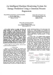
Q = number of FIR filter taps R = decimation prior to FIR filter stage τ = latency (µs) Fsamp = input sample rate of the FIR filter The latency of the FIR filter is determined by: τ = Q/Fsamp = (QR) / 50 MHz A Q vs R plot with a latency of 20 µs superimposed is shown in Figure 1.
2 DIGITAL DOWNCONVERTER (DDC) In an attempt to overcome limitations posed by analog electronics and non-ideal RF circuit elements, a digital scheme was proposed. The 1 MHz IF is oversampled by a 14-bit A/D running at 50 MSPS. Oversampling provides the benefit of reducing the quantization noise of the A/D converter by spreading the noise spectrum out to 25 MHz. The digitized signal is sent to a DDC, where the signal is heterodyned and decomposed to in-phase and quadrature (I & Q) components through the use of a numerically controlled oscillator (NCO) and quadrature multiplier. Subsequent narrowband Finite-Input-Response (FIR) filtering is required for a number of reasons: (i) to remove any residual aliasing components due to downconversion and decimation, (ii) to remove higher-order components *Work supported by the U.S. Department of Energy, contract DEAC05-84ER40150 †
[email protected]
0-7803-7191-7/01/$10.00 ©2001 IEEE.
Figure 1: Decimation, R, vs number of FIR taps (Q). 20µs latency contour added for reference.
2329
Proceedings of the 2001 Particle Accelerator Conference, Chicago An additional FIR requirement, specific to the Intersil HSP50214B DDC, is that the frequency of the FIR clock must exceed a minimum value to ensure completing a filter calculation before the result is required for output. This requirement[5] can be approximated by: Q ≈ 2(R-1) and appears as a straight line on the Q vs R plot (see Figure 1). The resulting latency and filter performance are plotted as Fstop vs R, and shown in Figure 2, where Fstop is the minimum stopband frequency of the FIR lowpass filter.
3 DIGITAL SIGNAL PROCESSOR (DSP) In addition to filtering provided by the DDC, a Texas Instruments TSM320C6711 DSP is employed to provide a means of filtering low S/N input signals, by varying the filter parameters in real-time to achieve a specific criteria (ie maximize S/N). This process is known as adaptive filtering or equalization.
3.1 Least-Mean Squares (LMS) Algorithm Adaptive filters have recently seen use in controls to filter out narrowband noise, as well as remove discrete sinusoid components. The most prevalent use of such filters is in the area of active noise cancellation within radio headsets and aircraft. These applications try to suppress the sinusoidal or coherent noise (such as from motors), while passing the incoherent noise. This BCM application attempts to preserve the sinusoidal tone, produced by intentionally mistuning the DDC NCO by 1 kHz. The schematic is commonly referred to an adaptive predictor, and is shown in Figure 3a. Predictor Topology yk Xk = S + N
(a)
+ ∆Τ
bk
FIR Filter
ek
−
LMS Algorithm
Identification Topology
Figure 2: Decimation, R, vs Latency and stopbandwidth, Fstop.
yk
The minimum value of R was calculated to be greater than 25, such that the output sample rate would be less than 2 MSPS. R should be a multiple of 2 to facilitate distribution between an onboard Cascaded Integrator Comb (CIC) and halfband filter. A value of R = 28 provided the most flexibility in implementation, as several factoring combinations are possible. The resulting FIR filter produced a filter having a latency of 20 µs, and 98kHz 3dB low-pass bandwidth. The final design values are summarized in Table 1. Table 1: FIR Filter Specifications Specification Value Decimation R 28 Passband Frequency Fpass 50 kHz Passband Attenuation Apass 0.1 dB Number of filter taps Q 36 Stopband attenuation Astop 70 dB Input sample rate
50 MHz /28 = 1.79 MHz
Stopband frequency Fstop
196 kHz
+
Xk = S + N IIR (Oscillator)
(b)
−
ek
LMS Algorithm
Figure 3: Adaptive prediction topology is shown at (a). Xk is input signal plus noise, while predicted and error signals are Yk and ek, respectively. FIR coefficients are denoted by bk. Adaptive Identification is shown in (b). FIR filter coefficients are found by the LMS algorithm which seeks to reduce the mean quadratic error, ek2, resulting from the difference between the actual signal and the best estimate of the signal. In theory, the ek contains only the stochastic signal contribution, while the filtered component, yk, is the deterministic component, or in this case, the 1 kHz tone: Let: Ck+1 = Ck - µGk Where Gk represents an estimate of the gradient vector, and Ck denotes an estimate of the vector of filter coefficients. µ is a step size (