As an example, consider the Morse-code alphabet. If length and length ... forschungsbereich F 003, Optimierung und Kontrolle, Projektbereich Diskrete. Optimierung. .... Recently, Bradford, Golin, Larmore, and Rytter [2] found a faster algorithm ...
1770
IEEE TRANSACTIONS ON INFORMATION THEORY, VOL. 44, NO. 5, SEPTEMBER 1998
A Dynamic Programming Algorithm for Constructing Optimal Prefix-Free Codes with Unequal Letter Costs Mordecai J. Golin, Member, IEEE, and G¨unter Rote
Abstract—We consider the problem of constructing prefix-free codes of minimum cost when the encoding alphabet contains letters of unequal length. The complexity of this problem has been unclear for thirty years with the only algorithm known for its solution involving a transformation to integer linear programming. In this paper we introduce a new dynamic programming solution to the problem. It optimally encodes n words in O (nC +2 ) time, if the costs of the letters are integers between 1 and C: While still leaving open the question of whether the general problem is solvable in polynomial time, our algorithm seems to be the first one that runs in polynomial time for fixed letter costs. Index Terms—Dynamic programming, Huffman code, optimal code.
I. INTRODUCTION
I
N this paper we present a new algorithm for constructing optimal-cost prefix-free codes when the letters of the alphabet from which the codewords are constructed have different lengths (costs). This algorithm runs in polynomial time when the costs are fixed positive integers, improving upon the previously best known algorithm which ran in exponential time even for fixed letter costs. Assume that messages consist of sequences of characters taken from an alphabet of source symbols and are transmitted over a channel admitting an encoding alphabet containing characters. The length of letter , length symbolizing its cost or transmission time, is A codeword is a string of characters in , i.e., The length of is the sum of the lengths of its component letters length
As an example, consider the Morse-code alphabet If length and length length
then
Manuscript received November 1, 1996; revised January 15, 1998. This work was supported in part by HK RGC/CRG under Grants HKUST 181/93E and HKUST 652/95E. The work of G. Rote was supported by the Spezialforschungsbereich F 003, Optimierung und Kontrolle, Projektbereich Diskrete Optimierung. The material in this paper was presented at the 22nd International Colloquium on Automata, Languages, and Programming (ICALP’95), Szeged, Hungary, July 1995. M. J. Golin is with the Computer Science Deptartment, Hong Kong UST, Clear Water Bay, Kowloon, Hong Kong. G. Rote is with the Institut f¨ur Mathematik, Technische Universit¨at Graz, A-8010 Graz, Austria. Publisher Item Identifier S 0018-9448(98)04644-6.
Codeword
is a prefix of codeword ) if and for A set of codewords all is prefix-free if no codeword is a prefix of another codeword A prefix-free code assigns a codeword to each of the source symbols, such that the set is prefix-free. For example, the codes and are prefix-free, whereas is not, because is a prefix of .A the code prefix-free code is uniquely decipherable, which is obviously a very desirable property of any code that is to be used. However, uniquely decipherable codes need not necessarily be prefix-free. be the probabilities with which the source Let symbols occur; these are also the probabilities with which the respective codewords will be used. The number is also The cost of called the weight or frequency of codeword is the code (with
length This is the expected length of the string needed to transmit one source symbol. and probaGiven integer costs the Optimal Coding Problem bilities containing prefix-free codewords with is to find a code minimum cost As an application, consider the case of runlength-limited codes, which is of importance for storage of information on magnetic or optical disks or tapes. The stored information can be viewed as a sequence of bits, but for technical reasons, it is desirable that the length of a contiguous block of zeros between two successive ones (a run of zeros) be bounded from above and below [20], [22]. For example, consider the -codes. We can model this in our common case of framework by combining each one-digit with the preceding block of zeros into a single character of our encoding alphabet
with associated lengths . Usually, the source symbols are taken as the symbols and with probabilities One can now take blocks of successive input bits and treat them as one source symbol. This gives source symbols with equal probabilities
0018–9448/98$10.00 1998 IEEE
GOLIN AND ROTE: PROGRAMMING ALGORITHM FOR CONSTRUCTING OPTIMAL PREFIX-FREE CODES
assuming that different input bits are distributed uniformly and independently. and then the length of codeword is If then just the number of characters it contains; if is the number of bits in , e.g., length length A minimum-cost binary code of this type is known as a time Huffman code and there is a very well known greedy algorithm due to Huffman [21] for finding such a code. This greedy algorithm cannot be adapted to solve the general optimal coding problem (in the next section we will see why). In fact, the only known solution for the general problem seems to be the one proposed by Karp when he formulated it in 1961 [14]. He recast the problem as an integer linear program, which he solved by cutting plane methods; this approach does not have a polynomial time bound. Since then, different authors have studied various aspects of the problem such as finding bounds on the cost of the solution [1], [13], [19] or solving the special case in which for all all codewords are equally likely to occur [5]–[7], [11], [15], [18], and [23], but not much is known about the general problem, not even if it is NP-hard or solvable in polynomial time. The only efficient algorithms known find approximately minimal codes but not the actual minimal ones [9]. In this paper we describe a dynamic programming approach to the general problem. In fact, our algorithm may be viewed as a dynamic programming solution of the integer programming formulation of Karp [14, Theorem 3]. Our approach is to construct a weighted directed acyclic graph with a polynomial number of vertices and arcs and demonstrate that an optimal code corresponds to a shortest path between two specified vertices in the graph. Finding an optimal code, therefore, reduces to a shortest path calculation. We first describe an algorithm that is easy to understand and time where is the largest runs in letter cost. We then improve the running time to For this second algorithm, some effort is required to prove its correctness. While our algorithms do not settle the long-standing question of the problem’s complexity they appear to be the first solutions that run in polynomial time for fixed letter costs. The two algorithms are both extremely simple and easy to implement; the bulk of the paper is devoted to deriving them and proving their correctness. The reader interested primarily in code is invited to skip directly to Figs. 5 and 6. The rest of the paper is structured as follows: in the next section we describe the problem in detail, showing how it can be transformed into a problem on trees. We then explain why the standard Huffman encoding algorithm fails in the general case. In Section III we introduce the procedure of truncating a tree at a given level, which allows us to transform the problem into shortest path construction on graphs. In Section IV we describe the improved algorithm. We conclude in Section V by describing implementation experiences, some open problems, and areas for future research. Recently, Bradford, Golin, Larmore, and Rytter [2] found a , using techniques faster algorithm for the binary case for finding minima in monotone matrices. The algorithm needs time. only
1771
Fig. 1. Two codetrees for five codewords using the three-letter alphabet 6 = f�1 ; �2 ; �3 g with respective letter costs c1 = c2 = 1 and c3 = 2: Part (a) encodes the set of words W = f�1 �1 ; �1 �2 ; �1 �3 ; �2 ; �3 g; and part (b) encodes the set W = f�1 �1 ; �1 �2 ; �2 �1 ; �2 �2 ; �3 g:
A shorter preliminary version of this paper was presented at the 22nd International Colloquium on Automata, Languages, and Programming in Szeged, Hungary [10]. II. SOME FACTS CONCERNING CODES AND TREES Throughout the remainder of the paper it will be assumed are fixed positive integers that the numbers are fixed positive reals. and be a prefix-free set of codewords. Let We will find it convenient to follow the standard practice and by an ordered, labeled tree By an ordered tree represent we mean one in which the children of a node are specified in a particular order. Each node in can have up to children, To build carrying distinct labels from the set of letters perform the following for each : start from the root and draw the path consisting of an edge labeled followed by an edge labeled followed by an edge labeled , an so on, until all characters have been processed. The th edge leaving a node corresponds to writing character in the codeword. See Fig. 1. ; This process will construct a tree corresponding to the tree will have leaves, each of which corresponds to a Note that a codeword cannot correspond to codeword in an internal node. This is because if the node corresponding appeared on a path leading from the root to a node to then would be a corresponding to another codeword prefix of , contradicting the prefix-free property. Also, note that this correspondence is reversible; every tree with leaves will correspond to a different prefix-free set of codewords. We draw our trees so that the vertical length of an edge is Such trees are also called lopsided trees in labeled , denoted by depth , the literature. The depth of a node is the sum of the lengths of the edges on the path connecting the root to the node. The root has depth . Note that if represents a code and a leaf represents then our length As usual, the definitions imply that depth height of a tree is the maximum depth of its leaves. is mapped to As an example, in Fig. 1(a) the codeword depth length , the leaf associated with and the tree has height . When we draw trees in this way, edge labels can be inferred from the edge lengths. (When several characters have the same length, we can assign labels arbitrarily without affecting the quality of the code.) In the sequel, we will therefore omit edge labels in the figures.
1772
IEEE TRANSACTIONS ON INFORMATION THEORY, VOL. 44, NO. 5, SEPTEMBER 1998
Suppose now that is a tree with leaves. Label the leaves as is the codeword assigned to the th input symbol, having probability Define the cost of the tree under the labeling to be its weighted external path length depth
cost
The following lemma is easy to see: be a fixed tree with Lemma 1: Let labeling of the leaves such that depth
depth
leaves. If
depth
is a
(1)
is minimum over all labelings of the tree. then cost which minProof: We want to find a permutation and imizes the inner product of two vectors depth where the entries of the second vector may be arbitrarily permuted. It is well known that the minimum is achieved by permuting one vector into increasing order and the other one into decreasing order, see [12, p. 261]. This lemma implies that in the optimal cost labeling the deepest node is assigned the smallest probability, the next deepest node the second smallest probability, and so on, up to the shallowest node which is assigned the highest probability (see Fig. 1). Such a code is called a monotone code, cf. Karp [14, Sec. IV]. Since we are interested in minimum-cost trees we will can restrict our attention to monotone codes. Thus cost be defined without specifying a labeling of the leaves because the labeling is implied by The Optimal Coding Problem is now seen to be equivalent and to the following tree problem: given find a tree with leaves with minimum cost over all trees with leaves, i.e., cost
cost
has
leaves
From here on we will restrict ourselves to discussing the tree version of the problem in place of the original coding formulation. For For example, in Fig. 1, we have the probabilities
the tree in Fig. 1(a) has minimum cost; for the probabilities
the tree in Fig. 1(b) has minimum cost. The corresponding codes are the optimal codes for those probabilities. Optimal trees have another obvious property: Lemma 2: In an optimal tree, every internal node has at least two children.
Proof: By contracting the edge between a node and its only child we would get a better tree. Before continuing, it is instructive to examine why the Huffman encoding algorithm for the case cannot be adapted to work in the general case. Recall that the Huffman encoding algorithm works by constructing the optimal tree from the leaves up. It assumes that it is given a collection of nodes with associated probabilities It takes the two leaves with lowest probability and combines them to form a new node with that it adds to the set while throwing probability away the two nodes it combined (for the rest of the algorithm those nodes will always appear as children of ). It then probabilities, stopping when recurses on the new set of the set contains only one node. A more complete description of the algorithm can be found in most introductory textbooks on algorithm design, e.g., [21]. Why does this algorithm work? Lemma 1 tells us that and can always be assigned to two deepest nodes in an optimal tree. In the standard Huffman case of a node and its sibling have the same depth and, in particular, the deepest node’s sibling is also a deepest node. Therefore, there is a minimum cost labeling of the optimal tree in which and are siblings of each the leaves assigned weights other. Algorithmically, this implies that these two leaves can be combined together as in the Huffman algorithm. , however, the deepest and In the general case when second deepest node are not necessarily siblings, and thus and cannot be combined, cf. Figs. 2 or 3.
III. A SIMPLE ALGORITHM
FOR
FULL TREES
We saw above that building the trees from the bottom up in a straightforward greedy fashion does not work. Instead, we have to consider many possible partial solutions, using a dynamic programming approach. In contrast to the bottom-up approach of the Huffman algorithm, we construct the trees from the top down, expanding them level by level. This, however, is not a necessary feature of our algorithm, it is only for ease of exposition. We construct a graph whose size is polynomial in and whose arcs encode the structural changes caused by expanding a tree by one level; the cost of an arc will be the cost added to the tree by the corresponding expansion. Trees will then correspond to paths in the graph with the cost of a tree being the cost of the associated path. An optimal-cost tree will correspond to a least cost path between specified vertices in the graph and will be found using a standard single-source shortest path algorithm. Before proceeding we must address a small technical point. Recall that we had reduced the Optimal Coding problem to the problem of finding a tree with leaves and minimal external path length. A tree is called a full tree if all of its internal nodes have any optimal the full set of children. For example, if this is tree must be full, by Lemma 2. Unfortunately, if no longer the case. See Fig. 2(a).
GOLIN AND ROTE: PROGRAMMING ALGORITHM FOR CONSTRUCTING OPTIMAL PREFIX-FREE CODES
1773
Fig. 2. A case in which r = 3; (c1 ; c2 ; c3 ) = (1; 1; 2). (a) An optimal tree T which is not full. (b) The augmented tree Fill (T ):
Fig. 3. A full tree T with depth 6, having seven internal nodes and 15 leaves. Each internal node has r = 3 children, and (c1 ; c2 ; c3 ) = (1; 1; 3):
For convenience, we will first present an easier version of the algorithm which assumes that the tree we are searching for is full.
have depth at most .
we denote the full Definition 1: Let be a tree. By Fill In other words, tree with the same set of internal nodes as to every internal node which has less than children, we add the appropriate number of children. These new leaves (the set are called the missing leaves of Fill
Fig. 3 gives a full tree and Fig. 4 shows its truncations to various levels. We will also need the following definition. is an -level tree if all internal Definition 3: The tree satisfy depth nodes
Since Fill may have more than leaves, we extend the definition of the cost of a tree by padding the sequence
The following are some obvious statements about truncation.
with sufficiently many zeros. This means that only leaves are selected with positive probability, and the remaining leaves are ignored in the computation of the cost. cost , because we We clearly have cost Fill with the same cost as can obtain an assignment for Fill by giving probability to the missing leaves. See cost Fig. 2(b). The restriction to full trees is therefore no loss of optimality. we use the fact of Lemma 2 To bound the size of Fill that every internal node of an optimal tree has at least two has at most internal nodes. A children. Therefore, full tree with internal nodes has leaves. The full tree that results from augmenting an optimal leaves. tree thus has at most We therefore recast the problem of finding the optimal leaves, and thus the optimal coding problem, as tree for and , set follows: given for and find the full tree with leaves , with minimum cost, i.e., cost
cost
has
leaves
It is this problem that we address now. After finding such a tree and peeling away its -probability nodes we will be left with the optimal-coding tree for leaves. We start by examining the structure of trees and how they can change as we expand them level by level. The basic tool we use is the truncated tree: Definition 2: Let be a tree and a nonnegative integer. containing The th-level truncation of is the tree Trunc the root of along with all other nodes in whose parents
Trunc
root
depth parent
Lemma 3: is an -level tree. • Trunc • If is an -level tree then Trunc • If is a full tree then Trunc is also a full tree. has at most as many leaves as • Trunc The idea behind our algorithm will be to build full trees from the top down. Given a tree with height we will start from a tree with just the root and successively build the Trunc where is the tree level trees containing only the root and its children and We will find that building from will not require but only a) the total number of leaves with knowing all of and b) the number of leaves of on depth at most in (There are no leaves beyond each level ) To capture this information we introduce the depth concept of a signature. of
Definition 4: Let be an -level tree. The -level signature is the -tuple sig
in which number of leaves in
is a leaf, depth with depth at most , and
is the
depth Even though the way in which sig is computed depends on the truncation level , the signature itself contains no Also note that the information identifying the value of truncation operation cannot increase the total number of leaves leaves and in the tree; so, if is a tree with at most then sig Trunc
1774
IEEE TRANSACTIONS ON INFORMATION THEORY, VOL. 44, NO. 5, SEPTEMBER 1998
Fig. 4. The trees T0 ; T1 ; T2 ; and T3 for r = 3; (c1 ; c2 ; c3 ) = (1; 1; 3): The dotted horizontal line is the sig level. Note that Trunc3 (T ) = Trunc4 (T ) = Trunc5 (T ) = Trunc6 (T ) = T , with sig4 (T ) = (11; 3; 1; 0); sig5 (T ) = (14; 1; 0; 0); and sig6 (T ) = (15; 0; 0; 0):
Suppose is the th-level truncation of some code tree for symbols with sig How much information concerning can be derived from ? are the same in First note that the nodes on levels and ; that is, if is a node with depth , then is a leaf in if and only if the corresponding node is a therefore has exactly leaves with depth leaf in We cannot say anything similar for a node in with depth greater than ; we know it is a leaf in but the corresponding might be an internal node. By Lemma 1, the node in largest probabilities in are assigned to the highest leaves highest leaves in All that is known in which are the probabilities is that they will concerning the remaining be assigned to nodes in that have depth greater than This leads us to the following definition. be an -level tree with sig Definition 5: Let For , the th-level cost of is depth
cost where depth. For
(2)
are the highest leaves of , we define
ordered by
depth
cost
The first term in the sum (2) reflects the cost of the paths leaves which have already been assigned, whereas to the the second term reflects only part of the cost for reaching the remaining leaves, namely, only the part until level Definition 6: Let i.e.,
Set
be a valid signature, to be the
minimum cost of a tree with signature precisely, cost
More is an -level tree
and sig If is an -level tree with sig and then, because for , we find that cost Also, contains at least cost nodes. Since we may restrict ourselves to trees which have at nodes the cost of the optimal tree is exactly the most where the minimum is minimal cost of and taken over all tuples in which An optimal tree is one that realizes this cost. To find this minimum value and its corresponding signature (and the tree with the signature that has that value) we use table. a dynamic programming approach to fill in the We will therefore investigate how truncated trees can be is an -level tree expanded level by level. Suppose that and is some -level with sig How can differ from ? tree with Trunc By the definition of Trunc , the two trees must be identical on levels through in that they contain the same nodes on those levels and a node is a leaf or internal in if and only if the corresponding node is respectively a leaf or internal Furthermore, the two trees contain exactly the same in because the parents of those nodes are nodes on level on level or higher. The only difference between the trees is the status of the nodes on that level. In on level , all of these nodes are leaves. In , some number of of them being leaves. Since them might be internal with , there are essentially possible -level with Trunc , a different tree corresponding trees Once is fixed, the number of to each possible value of
GOLIN AND ROTE: PROGRAMMING ALGORITHM FOR CONSTRUCTING OPTIMAL PREFIX-FREE CODES
nodes on levels through are also fixed since all such nodes are either nodes in or children of the internal of nodes at level This motivates the following definition: be an -level tree with sig Definition 7: Let Let The th expansion of at level is the tree Expand constructed by making of the leaves at level internal nodes with children.
of
Note that the definition does not specify which of the leaves become internal nodes in Expand For our purposes, however, this does not matter. Although different choices result in different trees, the number of leaves at each level is fixed, and more importantly, all resulting trees have the same cost. A formal statement of this fact requires a notion of equivalence between trees.
1775
Proof: Equation (3) follows directly from the discussion preceding the definition: on levels through has exactly On level has leaves. the same leaves as is therefore Nodes The first entry in sig of , for , were either appearing on level children on that level whose in tree or are one of the There are exactly of parents are on level of these. Finally, the only nodes appearing on level are the children of the internal nodes on level The proof of (4) follows from a similar analysis. Suppose ; otherwise, has obviously the same cost as The shallowest leaves in are exactly the same as the shallowest leaves in which are the leaves in at at depth or less. also contains exactly leaves at and its remaining leaves are all deeper than depth Thus with , we have depth
cost
and are equivalent if they Definition 8: Two trees have the same number of leaves at every level. We write this as depth The following lemma summarizes the obvious properties of this relation. Lemma 4: • All trees which may result as the th expansion of are equivalent. In other words, Expand level unique up to equivalence. , then Expand Expand • If provided that the expansions are defined. are two -level trees, then sig sig • If • If , then cost cost , for any
at is ,
cost Example 1: The following table signature
In order to describe the transformation of signatures affected by expansion, we need the characteristic vector associated to an alphabet with length vector : for is the number of that For example, are equal to
partial sums
shift level shift level
gives gives and gives Lemma 5: Suppose is an -level tree with sig Let Expand be its th expanThen is an -level tree with sion at level sig (3) where vector addition and multiplication by the scalar carried out componentwise (see Example 1 below), and cost
cost
is (4)
shows the transition from a signature to and by two and , respectively. We have expansions with and therefore The modification of the signature is done in two steps: the first step is the shift, which is due to the change of to level The second step is the focus from level addition of a suitable multiple of the vector which is given in the second line. The last column gives the which sequence of partial sums is important later. This last lemma tells us that to calculate the extra cost and the signature of the added by a level- expansion of new expanded tree it is not necessary to know or but only This motivates us to recast the problem in a graph sig formulation with vertices corresponding to signatures, arcs to expansions, and the cost of an arc to the cost added by its
1776
IEEE TRANSACTIONS ON INFORMATION THEORY, VOL. 44, NO. 5, SEPTEMBER 1998
associated expansion. A path in this graph will correspond to the construction of a tree by successive expansions; so an optimal tree will correspond to a least cost path of a certain type. More specifically, we define a directed acyclic graph , called the signature graph with
b) Let
be a path in
Let
be the root tree. Recursively define
Expand
(5)
Then the tree and
(6) and is a -level tree with cost Proof: a) First note that if sig
such that
We will often denote an arc by , indicating the value of that defines the arc. We also define a cost function on the arcs of
for
Fix . Since the Trunc operation cannot increase the as well. The arcs number of leaves in the tree, exist by the definition of the Trunc and Expand Straightforward calculation and operations. Thus yields the fact that cost
We pause here to point out the motivation behind this function. is an -level tree with sig and Suppose Expand with sig Then Lemma 5 tells us that
cost
cost
cost
cost
Note that the change in cost is independent of Now let be the tree containing only the root and its children. This tree, which we call the root tree, is the only -level full tree; so Trunc for every full tree Its sig is the starting signature vertex of the graph. For a directed path using arcs to get from to , we define the cost of the path in the usual way as the sum of the cost of its arcs, i.e.,
then
cost
cost
b) The fact that the exist and are -level trees with follows from the definition of the Expand sig operation. Equality of costs is obtained by following the above calculation backwards. We have just seen a) that every path of length in from to corresponds to a -level tree with and cost and b) that every sig -level tree corresponds to a -arc path from to with cost This proves the following sig lemma. and a minimum cost path from Lemma 7: Let to in Then If contains arcs and is as defined in (5) and (6) then cost
The following crucial lemma establishes a one-to-one corand respondence between paths of length emanating from -level trees with sig Lemma 6: be a -level tree with a) Let sig
The calculation of shortest paths is facilitated by the fact is acyclic (apart from possible loops at the that the graph ). We show this by specifying a specific vertices linear ordering of the vertices which is consistent with the orientation of the arcs (a topological ordering). Definition 9: Let
Set Trunc and let for
sig
be the number of internal nodes of Then the path
is contained in
, and
cost
at level
,
We define the linear order if and only if the vector
on the signatures so that
GOLIN AND ROTE: PROGRAMMING ALGORITHM FOR CONSTRUCTING OPTIMAL PREFIX-FREE CODES
1777
Fig. 5. The simple algorithm.
is lexicographically smaller than
For example, to compare and , we form their partial sums sequences and , respectively. We compare these vectors lexicographically, the rightmost entry and we being most significant. Since . In Example 1, the partial sums have sequence is indicated in the second column. It is quite easy to see that the signatures become bigger and bigger (in the “ ” order) by expansion. The shift of levels causes a left shift of the sequence, with the rightmost entry being duplicated, which is and then a multiple of the vector lexicographically positive, is added. Lemma 8: If Proof: Suppose
, and
then
and
If
, then
so If and
then Thus
and unless
for in which case
and For a directed acyclic graph , a shortest path can steps by scanning the vertices in be computed in topological order [16, p. 45]. We rewrite the algorithm for our special case and present it in Fig. 5. Note that in the algorithm but only we never explicitly construct the signature graph table implicitly use the graph structure to fill in the properly. In essence, we are performing dynamic programming
to fill in the table using an appropriate ordering of the table time entries. The algorithm takes for Steps 1 and 2a. Each vertex has outgoing arcs, and therefore Each time. Thus the total execution of Steps 2b and 2c takes time. cost of the algorithm is Note that the algorithm as presented only calculates the cost of the optimal tree. To actually construct the optimal tree, we have to augment the algorithm by storing a pointer with every is improved we array entry, and whenever update the pointer to remember where the current optimal value came from. (In fact it is sufficient to store the value which lead to the current value.) At the end we backtrack from the minimum-cost vertex to recover the optimal solution. This is standard dynamic programming practice, and we omit the details. IV. PRUNING
OF
EXTRA LEAVES
The algorithm in the previous section restricted its attention to full trees, i.e., trees in which every internal node contains all of its children. We had to pay for this convenience by leaves, many more constructing trees with as many as than the leaves actually used in the trees. In this section we improve the algorithm by looking only at trees with at most leaves, thereby reducing the complexity by a factor of Note that in the binary case of this makes no difference at all; the results of this section are only of interest when We have to relax the requirement of only constructing full trees, because optimal trees are not necessarily full, see, e.g., Fig. 2. This relaxation permits us to transform the construction of an optimal tree into a least cost path search in a new where signature graph
which has size and The design of the graph and the corresponding algorithm will be complicated by the following technical point: in the
1778
IEEE TRANSACTIONS ON INFORMATION THEORY, VOL. 44, NO. 5, SEPTEMBER 1998
previous section we constructed full trees level by level by specifying the number of internal nodes at each level. Since the trees being constructed were full, this specification uniquely determined the tree. If the trees are no longer required to be full then specifying the number of internal nodes on each level no longer uniquely specifies the tree; for each internal node it must also be known which children it has. As in the previous section, we want to construct the optimal tree level by level. However, if we ever generate more than leaves, we want to throw away some of them. It appears obvious that it is best to throw away the deepest leaves. In what follows we will prove that this is true. Definition 10: The reduction of a tree (to leaves) is the obtained by removing all but the shallowest tree Reduce leaves from It may happen that some internal nodes become leaves by this process because they lose all their children. In this case, we remove these additional “unwanted” leaves, and if necessary, we iterate this cleanup process. If does not have more than leaves, Reduce In other words, we can think of marking a set of shallowest leaves in The tree Reduce is then the unique subtree which has precisely this set of leaves. Similarly as in Definition 7, the set of leaves to be removed is not uniquely specified, but the number of leaves at each level is is unique up uniquely determined. In other words, Reduce to equivalence. It is obvious that reduction does not change the cost of a tree: Lemma 9: If
is an -level tree then cost Reduce
cost
Then sig Reduce reduce
Let
is defined as
Then there are leaving with
arc reduce
For each
Example 2: Below we show how Example 1 must be After each modified for the present section when expansion, we have to insert an additional reduction step. signature
partial sums
shift level reduce shift level reduce The reduction step is most easily understood in terms of the rightmost column: We simple reduce all partial sums which are bigger than to The modification of the main loop in the algorithm is straightforward. Step 2c is replaced by the following two steps. then replace 2c. If by reduce 2d. Set new cost
Proof: This follows from the fact that only the shallowest leaves affect the computation of the cost. If is an -level tree, then, in going from to Reduce , the signature changes as follows: Let sig Set For successively replace by
The modified signature graph follows:
The costs are as in the graph of Section III. The starting reduce , which vertex is the signature There is now also a unique corresponds to the root tree terminal vertex
arcs we have an
In the end, the cost of the optimal tree can be read off which corresponds to the terminal the entry vertex. is no longer acyclic, However, it turns out that the graph Therefore, it is not see Example 2, where we have obvious that the above modification is enough to compute the shortest path. However, by studying the example carefully we need not worry see why such “backward arcs” like to three leaves at level become us. In going from internal nodes, causing nine leaves to be added to the tree. But the following reduction chops off all but three of these new leaves. This means that at least one of the three new internal nodes has only one child remaining, but, by Lemma 2, such a node cannot occur in an optimal tree. To prove correctness, we need to show two things. First, to every path in the graph from the starting vertex corresponds to some tree, with appropriate cost. Secondly and more importantly, the optimal tree corresponds to which visits the vertices in an order to a path from These crucial proconsistent with the lexicographic order perties are formulated in the following lemma, which is an analog of Lemma 6. Lemma 10: be an optimal tree with height denoted by a) Let Set Trunc Reduce Fill sig and let be the number of internal , for Then nodes of at level
GOLIN AND ROTE: PROGRAMMING ALGORITHM FOR CONSTRUCTING OPTIMAL PREFIX-FREE CODES
the path
If we apply the reduction operation to both sides of this equation, we obtain
exists in
Reduce Fill
, with
and b) Let
cost
be a path in define
Let
be the root tree. Recursively
Reduce Expand
Then the tree is a -level tree with cost Proof: a) Note first that in as well as in each , every missing leaf has depth at least : if a missing leaf of had depth less than , we could remove some leaf at level and add a new leaf in the position of the missing leaf, obtaining a better tree. Since the truncation operator deletes either all children of a node or none, it generates no new missing leaves. Therefore, The the claimed property carries over from to all trees following property follows: Property 1: In all trees Fill depth less than is less than Optimality of
To prove the lemma we must show that Reduce Expand We will use the fact that Expand Fill
(7)
This is true because both trees are full trees which have the same number of internal nodes at each level. has Let us first deal with the easy case where Fill leaves. Then the reduction operation is void, less than Fill and we have Expand Fill
Reduce Expand Fill
Expand
Reduce Expand
By applying (7) we obtain Reduce Fill Reduce Expand Fill Reduce Expand which is what we wanted to show. , let To show
implies another property.
Proof: If , then a node at level can have at most one child in the tree By Lemma 2, a node with one child cannot occur in an optimal tree, and hence there are no internal nodes at level On the other hand, if , then at least two children of each node that is expanded lie on levels and these children more than compensate for the loss of leaves that are expanded due to the fact that the leaves at level become internal nodes.
Fill
Reduce Expand
which is what we wanted to show. We also have because either has more leaves in total than (in case ), or the reduction operation is void also for Fill In the latter case we have Expand , and we can apply Lemma 8. has Now let us consider the other case, where Fill leaves. By Property 1, Fill has less than at least leaves at levels The same is true for Reduce Fill and therefore has height Fill and Reduce Fill have the same number of leaves , and both trees have at least at each level between and leaves in total at levels After expansion, it follows and Expand that also the trees Expand Fill have the same number of leaves at each level between and and, moreover, by Property 2, both trees still have at least leaves in total at levels The reduction operation will therefore yield equivalent trees
, the number of leaves at
, then , and the operation Property 2: If increases the total number of leaves at levels Expand
Fill
1779
sig and sig By the above considerations about the numbers of leaves at levels up to , we have and but we have for (Note is the signature at level ) Thus that b) Since the Expand and Reduce operations are faithfully modeled by the arcs of the graph, it follows that the trees exist and have the given signatures. Equality of costs can be proved in the same way as in Lemma 6, using the fact that reduction does not influence the cost (Lemma 9). Thus as in the previous section, we can actually find the steps, each step shortest path in time. The code is given in Fig. 6. Actually, it is taking not difficult to be more careful in the implementation and avoid scanning the “backward arcs” of the graph. In the loop of Steps 2b–2d, we let run only up to We leave it as an exercise for the reader to check that this is correct. for the number of nonnegative The bound -tuples with
1780
IEEE TRANSACTIONS ON INFORMATION THEORY, VOL. 44, NO. 5, SEPTEMBER 1998
Fig. 6. The improved algorithm.
is only a loose estimate. By looking at the strictly increasing sequence (8) we see that these tuples are in one-to-one correspondence -subsets of the set with the family of and hence their number is (In fact, if one wants to as compactly as possible, in an array of store the table entries in the proper lexicographic order , it is most convenient to use the vector (8) for indexing.) The number of , and the processing of each arc arcs is now time. This gives a time involves an overhead of bound of
We have for all as can be easily proved by induction on , proving the base and separately. We have therefore proved cases the following theorem. Theorem 1: The minimum-cost prefix-free code for words can be computed in time and space, if the costs of the letters are integers between and V. CONCLUSIONS, IMPLEMENTATIONS,
AND
OPEN PROBLEMS
In this paper we described how to solve the optimaltime where the letter lengths coding problem in are integers, is the longest length of an encoding letter, and is the number of symbols to be encoded. This improves upon the previous best known solution due to Karp [14] which solved the problem by transformation to integer linear programming and whose running time could therefore only be bounded by an exponential function of Our algorithm works by creating a weighted graph with vertices and arcs and showing that
optimal codes (corresponding to minimum cost trees) can be constructed by finding least cost paths in It is easy to see that the height of a tree is exactly the number to Thus we can of arcs in its corresponding path from also use our formulation to solve the Length-Limited Optimal Coding Problem. In this problem, we are given the same data as in the original problem and an integer , and we want to find a minimum-cost code containing no codeword of length To solve this new problem it is only necessary is more than to find the least cost path from the source to the sink that uses or fewer arcs, which can be easily done in time. In a practical implementation of our algorithm many improvements are possible. Recall that our algorithm is equivalent to searching for a shortest path in a directed acyclic graph. The simple shortest path algorithm which we used essentially scans all arcs of the graph. There is a whole range of heuristic graph search algorithms to be considered that might speed up the running time of the algorithm in practice, cf. [17]. One obvious direction for future research is to resolve the complexity of the optimal-coding problem. It is still unknown if the problem is polynomial-time solvable, or if the problem is NP-hard. are Another direction is to relax the restriction that the integers. Obviously, in any conceivable practical application are rationals; therefore, they can all the given numbers be scaled to be integers and our algorithm can be used. However, since the largest integer cost enters into the exponent of the complexity, this approach is in general not feasible. It is challenging to find an algorithm that would solve the problem with, for example, in reasonable time, and which could just as easily be applied to incommensurable lengths such as It is not known whether the restriction to prefix-free codes in the optimal coding problem, as opposed to the more general class of uniquely decipherable codes, is a severe restriction that excludes codes which would otherwise be optimal, or whether an optimal code in the class of uniquely decipherable codes can always be found among prefix-free codes. See the survey by Bruy`ere and Latteux [4] for this and related open problems.
GOLIN AND ROTE: PROGRAMMING ALGORITHM FOR CONSTRUCTING OPTIMAL PREFIX-FREE CODES
We have tested the algorithm for computing optimal codes for the Roman alphabet plus “space,” using the probabilities which are given in [3, p. 52] and reproduced in Karp [14]. We ran an experimental implementation of our algorithm in MAPLE on an HP 9000/750 workstation. When the encoding , we found an optimal alphabet had two letters, in 1.5 s. For an encoding alphabet code with a cost of , we found an optimal with three letters, in 6 s. The only algorithm in the literature cost of for which running times are reported is the algorithm of Karp [14] from 1961. His program took 1 min for the first example and 5 min for the second one on an IBM 704 computer. (The code we found for the first example was different from Karp’s even though, of course, it had the same cost.) These running times can hardly be compared. On the one hand, this machine was much slower than today’s computers. An IBM 704 in 1955 could carry out about 5000 floating-point operations per second (0.005 MFLOPS). On the other hand, the MAPLE system is not designed for taking the most efficient advantage of computer hardware. For example, all arithmetic operations are carried out in software, and array indexing is not as efficient as in a conventional programming language. (For the second problem, about 40% of the total running .) We ran an integer time was spent initializing the array programming formulation derived from Karp’s on the same workstation as our MAPLE code. The model was formulated in the AMPL modeling language [8], using about 25 lines of code, and was solved with the CPLEX 4.0 software for mixed-integer optimization. Interestingly, the three-letter problem was easier to solve than the two-letter problem. It took 0.19 s, 46 branchand-bound nodes, and a total of 207 pivots of the simplex algorithm to solve the two-letter problem, but only 0.09 s, 3 branch-and-bound nodes, and 143 simplex iterations to solve the three-letter problem. ACKNOWLEDGMENT The authors wish to thank Dr. Jacob Ecco for introducing them to the Morse Code puzzle which sparked this investigation.
[3] [4]
[5]
[6] [7] [8] [9] [10]
[11] [12] [13] [14] [15] [16] [17] [18] [19] [20]
REFERENCES [21] [1] D. Altenkamp and K. Mehlhorn, “Codes: Unequal probabilities, unequal letter costs,” J. Assoc. Comput. Mach., vol. 27, no. 3, pp. 412–427, July 1980. [2] P. Bradford, M. J. Golin, L. L. Larmore, and W. Rytter, “Optimal prefixfree codes for unequal letter costs and dynamic programming with the
[22] [23]
1781
Monge property,” to be published in Algorithms. Proc. 6th Europ. Symp. Algorithms (ESA ’98), G. Bilardi and G. F. Italiano, Eds. (Lecture Notes in Computer Science). Berlin, Germany: Spsringer-Verlag, 1998. L. Brillouin, Science and Information Theory. New York: Academic, 1956. V. Bruy`ere, and M. Latteux, “Variable-length maximal codes,” in Automata, Languages and Programming, Proc. 23rd Int. Colloq. Automata, Languages, and Programming (ICALP 96), F. Meyer auf der Heide and B. Monien, Eds. (Lecture Notes in Computer Science, vol. 1099). Berlin, Germany: Springer-Verlag, 1996, pp. 24–47. S.-N. Choi and M. Golin, “Lopsided trees: analyses, algorithms, and applications,” in Automata, Languages and Programming, Proc. 23rd Int. Colloq. Automata, Languages, and Programming (ICALP 96), F. Meyer auf der Heide and B. Monien, Eds. (Lecture Notes in Computer Science, vol. 1099). Berlin, Germany: Springer-Verlag, 1996, pp. 538–549. N. Cot, “A linear-time ordering procedure with applications to variable length encoding,” in Proc. 8th Annu. Princeton Conf. Information Sciences and Systems, 1974, pp. 460–463. , “Complexity of the variable-length encoding problem,” in Proc. 6th Southeast Conf. Combinatorics, Graph Theory and Computing, 1975, pp. 211–224. R. Fourer, D. M. Gay, and B. W. Kernighan, AMPL: A Modeling Language for Mathematical Programming. Danvers, MA: Boyd & Fraser, 1993. E. N. Gilbert, “Coding with digits of unequal cost,” IEEE Trans. Inform. Theory, vol. 41, pp. 596–600, Mar. 1995. M. Golin and G. Rote, “A dynamic programming algorithm for constructing optimal prefix-free codes for unequal letter costs,” in Automata, Languages and Programming, Proc. 22nd Int. Colloq. Automata, Languages, and Programming (ICALP 95) (Szeged, Hungary, July 1995), F. G´ecseg, Ed. (Lecture Notes in Computer Science, vol. 944). Berlin, Germany: Springer-Verlag, 1995, pp. 256–267. M. J. Golin and N. Young, “Prefix codes: equiprobable words, unequal letter costs,” SIAM J. Computing, vol. 25, no. 6, pp. 1281–1292, Dec. 1996. G. H. Hardy, J. E. Littlewood, and G. P´olya, Inequalities. Cambridge, U.K.: Cambridge Univ. Press, 1967. S. Kapoor and E. Reingold, “Optimum lopsided binary trees,” J. Assoc. Comput. Mach., vol. 36, no. 3, pp. 573–590, July 1989. R. Karp, “Minimum-redundancy coding for the discrete noiseless channel,” IRE Trans. Inform. Theory, vol. IT-7, pp. 27–39, Jan. 1961. A. Lempel, S. Even, and M. Cohen, “An algorithm for optimal prefix parsing of a noiseless and memoryless channel,” IEEE Trans. Inform. Theory, vol. IT-19, pp. 208–214, Mar. 1973. K. Mehlhorn, Data Structures and Algorithms 2: Graph Algorithms and NP-Completeness. Berlin, Germany: Springer-Verlag, 1984. N. J. Nilsson, Principles of Artificial Intelligence. Palo Alto, CA: Tioga, 1980. Y. Perl, M. R. Garey, and S. Even, “Efficient generation of optimal prefix code: Equiprobable words using unequal cost letters,” J. Assoc. Comput. Mach., vol. 22, no. 2, pp. 202–214, Apr. 1975. S. A. Savari, “Some notes on Varn coding,” IEEE Trans. Inform. Theory, vol. 40, pp. 181–186, Jan. 1994. K. A. Schouhamer Immink, “Runlength-limited sequences,” Proc. IEEE, vol. 78, pp. 1744–1759, 1990. R. Sedgewick, Algorithms, 2nd ed. Reading, MA: Addison-Wesley, 1988. P. H. Siegel, “Recording codes for digital magnetic storage,” IEEE Trans. Magn., vol. MAG-21, pp. 1344–1349, 1955. L. E. Stanfel, “Tree structures for optimal searching,” J. Assoc. Comput. Mach., vol. 17, no. 3, pp. 508–517, July 1970.