An Adaptive Dynamic Programming Algorithm for ... - CiteSeerX

An Adaptive Dynamic Programming Algorithm for Dynamic Fleet Management, I: Single Period Travel Times Gregory A. Godfrey • Warren B. Powell

Department of Operations Research and Financial Engineering, Princeton University, Princeton, New Jersey 08544

W

e consider a stochastic version of a dynamic resource allocation problem. In this setting, reusable resources must be assigned to tasks that arise randomly over time. We solve the problem using an adaptive dynamic programming algorithm that uses nonlinear functional approximations that give the value of resources in the future. Our functional approximations are piecewise linear and naturally provide integer solutions. We show that the approximations provide near-optimal solutions to deterministic problems and solutions that significantly outperform deterministic rolling-horizon methods on stochastic problems.

We consider the problem of assigning a set of homogeneous vehicles (or resources) to customer demands (or tasks) that arise randomly over time. Each vehicle is in a particular state (typically, a geographical location), and each task requires a resource in a particular state. The assignment of a resource to a task generates revenue and removes the task from the system. It also changes the state of the resource. A resource in one state can be transformed into a resource in selected other states at a cost. A task may be assigned to resources in a specified subset of states. Finally, we assume that all transitions require one time period (such as four hours or a day). Needless to say, we are generally interested in integer solutions to this problem. Our problem arose in the context of managing fleets of vehicles that are allocated spatially over time. Vehicles might be trailers, boxcars, or containers, or they may be rental cars and trucks. The same problem structure also arises in machine scheduling with setups (moving a truck from one city to the next is identical to a machine with a setup cost and time), as well as other forms of resource transformation (such as personnel training). Even in transportation, 0041-1655/02/3601/0021$05.00 1526-5447 electronic ISSN

the movement of a vehicle from one location to the next may involve more than a change in space: the truck may have less fuel; the driver may have reduced hours of service; and a chemical trailer may become dirty and, therefore, may need to be cleaned. We refer to this problem as the stochastic dynamic resource allocation problem (SDRAP), a problem class with its roots in fleet management. It arises in a variety of settings, including: fleet management (how many empty box cars or trailers should be moved empty from one location to the next and which loads should be served first), car rental fleets (how many rental cars, and which types, should be assigned to a particular pool), dynamic crew scheduling (assigning drivers to move loads from origin to destination, taking into account all the characteristics of each type of driver), training of military personnel (how many recruits should receive a particular type of specialty training), and remnant inventory (given bins of pipes of different lengths, we wish to choose a pipe that is at least as long as the required demand, cut it down to the needed size, and then put the leftover piece in the appropriate bin). Transportation Science © 2002 INFORMS Vol. 36, No. 1, February 2002 pp. 21–39

GODFREY AND POWELL Single Period Travel Times

• Queues of tasks and resources at each location in the network • Resources move to service a task or reposition

• Tasks must be serviced within time window to receive full revenue • Over time, new tasks arrive, old tasks expire Resources Service Task Figure 1

Tasks Reposition

Physical Depiction of Dynamic Resource Allocation Problem

An illustration of the problem in a spatial context is given in Figure 1. Here, we have a set of points in space, and at each point are a queue of resources waiting to be assigned and a queue of tasks waiting to be completed. Each task will require moving a resource from one location to another. We have to decide which resources to assign to which tasks, and if we have excess resources, whether we want to transform (or in this setting, move) any resources from one location to another. Three issues make solving this problem more interesting than simply matching resources to tasks at a common location. First, the planner may pay a cost to transform a resource from one state to another (for example, a change in location, cleaning a chemical trailer, or taking a driver off-duty). We call this repositioning the resource. Second, a planner may be penalized (receive a reduced revenue) for servicing a task too late. We define the task time window as the time during which a task may be serviced at full revenue (the reward function may be relatively complex). Third, over time, new resources and tasks become available via some random process. This mimics the real-world process of people calling for taxis or customers calling to have packages picked up. Although the planner cannot know the exact future, we assume that historical information is available about the demand process and can be used to estimate probability distributions. This paper fills a gap in the research literature. Traditional dynamic programming methods focus on discrete state and action spaces (Puterman 1994). 22

Forward dynamic programming using Monte Carlo methods (Bertsekas and Tsitsiklis 1996, Sutton and Barto 1998) is not as sensitive to large state spaces, but does suffer from large action spaces (they generally require the ability to search the entire action space to choose the best one). Forward dynamic programming methods also require the ability to estimate the value of the system being in a particular state. However, convergence proofs are only available under very strong assumptions (in particular, that each state will be visited infinitely often); in practice, we only visit the states generated by a particular policy, and if we produce a poor estimate of the value of a state, we may never again choose the actions that return us to this state. A different line of investigation is to draw on the theory of stochastic linear programming (see the recent books by Infanger 1994, Kall and Wallace 1994, and Birge and Louveaux 1997). This literature can be divided between two-stage linear programs and their extension to multistage problems. Two-stage stochastic programs have been formulated as large-scale optimization problems subject to nonanticipativity constraints (Dantzig 1955, Rockafellar and Wets 1991), but these approaches typically limit the size of the problem we can consider. Techniques have been developed that approximate the second-stage recourse function (using either a static sample or with dynamic sampling). Approximations can be made through linearization methods (Ermoliev 1988, Ruszczynski 1980) or through the use of Benders cuts, which may be generated from a static sample (Van Slyke and Wets 1969) or dynamically through sampling-based methods (Higle and Sen 1991). Linearization methods usually benefit from nonlinear terms that stabilize the behavior. Examples include auxiliary function methods that combine stochastic gradient information with nonlinear stabilizing terms (Culioli and Cohen 1990, Cheung and Powell 2000) or proximal point terms (Ruszczynski 1987). These techniques are relevant to this research because it is always possible to take an approximation algorithm that is convergent for twostage problems and apply it heuristically to a multistage problem. Multistage problems are particularly problematic. Birge (1985) presents a nested Benders algorithm Transportation Science/Vol. 36, No. 1, February 2002


for multistage stochastic programs, but the method is impractical for even medium-sized problems. Monte Carlo-based methods mitigate the difficulty of working with large sample spaces. Higle and Sen (1991) introduced the first sampling-based methods for two-stage stochastic programs. Pereira and Pinto (1991) suggest a sampling-based version of nested Benders decomposition (without a proof of convergence). Chen and Powell (1999) propose a convergent sampling-based version of nested Benders for multistage problems with independence across stages. Unfortunately, all of these methods depend on Benders cuts to approximate the impact of decisions on future time periods. This general approach suffers from extremely slow convergence for problems with even a modest number of dimensions. In addition, integrality constraints are problematic. A number of approximations have been proposed in the context of fleet management, which represents a classic stochastic resource allocation problem. Jordan and Turnquist (1983) and Powell (1986) present methods for continuous (noninteger) flows. Powell (1987), Frantzeskakis and Powell (1990), Cheung and Powell (1996), and Powell and Carvalho (1998) present approximations that naturally produce integer solutions. Most of this work (Powell 1987, Frantzeskakis and Powell 1990, Cheung and Powell 1996) was not designed for problems with time windows (tasks that may be serviced over a range of time periods). The best results from this line of research are given in Cheung and Powell (1996), but these techniques are also relatively difficult to apply. Most recently, Carvalho and Powell (2000) propose a linear approximation with a multiplier adjustment procedure (LAMA) that works only on deterministic problems but gives promising results. Our approach to solving this problem uses the CAVE (Concave Adaptive Value Estimation) algorithm of Godfrey and Powell (2001) to construct a concave, separable, piecewise-linear approximation of the value function that is more flexible and responsive than linear approximations. Previously, CAVE had been applied only to two-stage problems, but we apply it to multistage problems with single period travel times. The travel time assumption simplifies Transportation Science/Vol. 36, No. 1, February 2002

the mathematical presentation and avoids issues specific to multiperiod travel times that are beyond the scope of this paper. Readers are referred to Godfrey and Powell (2002) for a treatment of the problem with multiperiod travel times. The contribution of this paper is a novel approximation strategy for solving multistage stochastic resource allocation problems. We avoid the curse of dimensionality of dynamic programming and the complexities associated with solving multistage stochastic linear programs using classical scenario methods. The method is computationally very fast and appears to produce near optimal solutions for deterministic problem instances. Most significantly, it outperforms rolling-horizon procedures, which represent the state of the art for engineering practice for this problem class. In §1, we present the notation and formulate the problem as a dynamic program. Then, §2 describes our solution strategy, where we use a novel approach for approximating dynamic programs for multistage linear programs. Section 3 describes methods for producing nonlinear approximations of value functions using gradient information, including a summary of the CAVE algorithm used to construct piecewise linear concave approximations of the value function. In §4, we show how to apply the CAVE logic to solve multistage dynamic programs. Section 5 presents a series of deterministic and stochastic experiments that test our proposed algorithm over a wide range of data sets. Finally, in §6, we present our conclusions to the research.

1.

Notation and Problem Formulation

In this section, we define the notation and problem dynamics for modeling the SDRAP over a fixed finite planning horizon. We have adopted the standard notation suggested by Powell et al. (2002), simplifying when possible and adding stochasticity where necessary. We conclude with a recursive dynamic programming formulation of the problem.

23


The Network The physical and temporal elements of the underlying transportation network are defined as follows. T = the number of planning periods in the planning horizon. = 0 1 T − 1, the times at which decisions are made. = the set of physical locations in the network, indexed by i and j. We model the problem in discrete time, reflected in the set . In practical applications, we find that it is necessary to represent the exact time within a time period, but for the purposes of this paper, we represent all activities as beginning and ending at a particular instant in the set . A critical assumption in this paper is that the time required to move between any pair of locations is a single time period.

l = the set of time periods over which task l may be served. If the task is not served within this interval (the time window), then it is assumed lost. Our care in distinguishing between the sets t+ and t becomes important later when we define our state variable. Note that t is empty if all tasks must be served at a single point in time. This observation is pertinent when we compare experiments where all the tasks must be served at a point in time to those where there are time windows. t t represent the new information Let Wt = R arriving in time period t. Wt Tt=0 is our stochastic information process, with realization Wt = t = t t . Let t be the -algebra generated by

R

W0 Wt , with = T . Then our probability space is given by , where is a probability measure defined on .

Resources and Tasks At the beginning of the planning horizon, there is an initial set of tasks to be performed and an inventory of resources available to perform the tasks. All resources are the same, and any resource may serve any task as long as they are at the same location. Over time, additional resources may become available for the first time. For each t ∈ , i ∈ , we define it = the number of resources that first become R it i∈ ; t = R available at location i at time t, with R Rit = the total number of resources available at location i at time t before any new arrivals have been added in, with Rt = Rit i∈ ; R+ t = the total number of resources that are availt ; able to be used in time period t = Rt + R To keep track of the available tasks, we define: t = the set of tasks that first become available in time period t; t = the tasks available at time t before the new t are added to the system; arrivals in + t = the set of tasks available to be serviced at time t, including new tasks that just arrived in this t ; period = t ∪ + it = the set of tasks that must be served by resources in state i (t+ = i∈ it+ ); b = the vector of attributes of task ∈ t+ . We assume that the sequence b ∈ is drawn from a known distribution;

Decision Variables At each time period, a resource must service a task, reposition, or sit idle. To service a task, we assume that the resource and task are matched at the task origin and then move to the task destination. A resource repositions simply by moving from one location to another. The decision to sit idle is equivalent to a reposition from location i to location i that takes one period to complete (a reposition across time, but not space). To formalize these decisions, we define for each t ∈ , i j ∈ and l ∈ t+ ,   1 If a resource is assigned to a task l ∈ t+ at time t xlt =  0 otherwise,

24

yijt = The number of resources repositioned from i to j beginning at time t. We also define the vectors xt ≡ xlt l∈t+ and yt ≡

yijt i j∈ . State Variables The relevant history of our system is captured by the state variable, giving the set of available resources and tasks: + St+ = R+ t t Transportation Science/Vol. 36, No. 1, February 2002


We have not found this version of the state variable to be the most useful. As an alternative, we define: St = Rt t We refer to St as an incomplete state variable because it does not contain all the information required to make a decision. In the special case that all tasks must be served immediately or they are lost, the set t is empty (because it does not yet include the new t ). In general, t includes only the tasks arrivals left over from previous time periods, which in many problems is relatively small. Note that our decisions

xt yt are t -measurable functions. Since St+ includes Wt , xt yt are random variables if we only know St . We note that St is an t−1 -measurable function. In the future, we may write St+1 , and it needs to be understood that this is a function of 0 1 t or, in our case, simply t . Objective Function The cost parameters used to evaluate decisions are cij = the cost to reposition a resource from location i to location j; rlt = the reward received for servicing task l ∈ t+ starting at time t ∈ . The decision to sit idle is represented by yii at a cost cii (which is often zero). Let gt xt yt be the one-period reward function: gt xt yt = rlt xlt − cij yijt i∈ l∈ + it

i∈ j∈

= the total profit gained from the decisions made at time t.

(1)

We let the feasible region t at time period t for a given outcome be given by: it ∀ i ∈ (2) yijt + xlt = Rit + R j∈

l∈it+

xlt ≤ 1

∀ l ∈ t+

(3)

xlt ≥ 0

t+

(4)

yijt ≥ 0

∀l ∈

∀ i j ∈

(5)

In addition, we have to express the dynamics of the system over time. For this purpose, we first need to Transportation Science/Vol. 36, No. 1, February 2002

define the set of tasks which are served: te xt = the tasks that expire in time period t, either because they are served or they hit the end of the time window. The dynamics of the resources and tasks are then given by:

t+1 = t+ \ te

Rj t+1 = yijt + xlt i∈

(6) ∀ j ∈ (7)

+ l∈ijt

The objective is to maximize expected profits over the T -stage planning horizon given an initial state S0 . We may write the problem as:

max g0 x0 y0 + E max gt xt yt (8) x0 y0 ∈0

t∈ \0

xt yt ∈t

The functions gt , decisions xt yt , and constraints t are all t -measurable functions. The system dynamics are given by Equations (6)–(7). Of course, we now face the problem of solving this formulation.

2.

Solution Strategy

In practical applications for this problem class, the most natural solution strategy is to use a rollinghorizon procedure, solving the problem at time t using what is known at time t and a forecast of future events over some horizon. Our goal is to produce a method that outperforms this basic approach. We begin by writing the optimality equations using Bellman’s principle of optimality. For this purpose, we have to choose how to represent the state of our system. If we use St+ , then we have all the information + we need to make decisions at time t; St+1 is random only because it includes the new information arriving in time period t +1. Using this formulation, we would obtain the recursion: + + Vt+ St+ = max gt xt yt + E Vt+1

St+1 St+ (9)

xt yt ∈t

In this formulation, the expectation is conditioned on the prior state St+ . We refer to Vt+ St+ as the value function and assume a terminal reward of VT+ · = 0. The problem with Equation (9) is that it is not computationally tractable. In this form, it suffers from the 25


three curses of dimensionality: the state space, the outcome space, and the action space. We solve these problems in the following way. First we reformulate the optimality equations in terms of the incomplete state variable: (10) Vt St = E max gt xt yt + Vt+1 St+1 St

xt yt ∈t

This allows us to drop the expectation and solve the problem for a single sample realization: Vt St =

max

xt yt ∈t

gt xt yt

+ Vt+1 St+1

(11)

If we had retained the original formulation using the complete state variable, dropping the expectation would have meant that we were solving the problem for a sample realization t+1 , which would mean that we would be choosing xt using t+1 , a violation of the measurability of our decision function. It is important to remember that St+1 is t -measurable. Finally, we replace the value function Vt+1 St+1 t+1 Rt+1 that depends with an approximation V t+1 Rt+1 purely only on the resource vector. Writing V as a function of Rt+1 (and excluding t+1 ) is an approximation that will introduce errors, but it simplifies the algorithm considerably and, as we show below, produces very good results. This gives us: t Rt = V

max

xt yt ∈t

gt xt yt

t+1 Rt+1 +V

(12)

t Rt serves as a placeholder. This problem where V is solved subject to: it ∀ i ∈ (13) yijt + xlt = Rit + R j∈

i∈

l∈it+

yijt +

+ l∈ijt

xlt = Rj t+1

∀ j ∈ (14)

xlt ≤ 1

∀ l ∈ t+

(15)

xlt ≥ 0

t+

(16)

∀l ∈

yijt ≥ 0 ∀ i j ∈

(17)

The first constraint (13) enforces conservation of flow by specifying that each resource at location i at time t 26

must either reposition (yijt ) or service a task (xlt ) (since we are implicitly conditioning on St , we do not index Rit by ). Constraint (14) counts how many resources move to location j at time t + 1. Constraint (15) specifies that each task cannot be assigned more than once. Constraints (16) and (17) are the requisite nonnegativity constraints. We now face the challenge of devising a suitable t Rt . The simplest approximation is approximation, V a linear one, but these can be unstable. Instead, we prefer to use a nonlinear (piecewise linear) separable approximation that we express as: t Rt = V

i∈

it Rit V

(18)

Our choice of this approximation is motivated by two issues. First, it is possible to show that the real value function is piecewise linear and concave with respect to Rt . This property follows from the wellknown result that a nonlinear program with concave objective function is a concave function of the linear right-hand-side constraint vector (see Rockafellar 1972). Second, as we illustrate later, this form of approximation means that Equations (12)–(17) form a network problem. If we ensure that the breakpoints of it Rit occur at integer the piecewise linear function V values of Rit , then the solution of our approximate subproblem is also guaranteed to be integer. In the next section, we describe the algorithm that it Rit using dual information we use to estimate V obtained from solving our sample subproblem.

3.

Fitting Concave Functional Approximations

In the previous section, we formulated a dynamic program using a separable concave approximation of Vt Rt . In this section, we describe methods for estimating functions of this type. We assume that we can readily compute a valid stochastic subgradient v ∈ V R or, in special cases, left and right derivatives that we denote: v+ = V R + 1 − V R v− = V R − V R − 1 Transportation Science/Vol. 36, No. 1, February 2002


Since V R is a concave function, we obtain the property that v− ≥ v+ . At each iteration n of our algorithm, we sample the variable Rn , then choose a sample observation n and calculate the slope vn n (or possibly the left and right gradients vn− n and vn+ n ) of the function V R for R = Rn . Given this information, we want to update our estimate of n R to obtain a new concave a concave function V n+1 estimate V R. There is a family of algorithms for estimating piecewise linear concave functions from stochastic subgradients which maintain concavity at each iteration. In our numerical experiments we use the CAVE algorithm of Godfrey and Powell (2001), but the technical details of this algorithm, while useful in practical experiments, disguise the essential ideas. For this reason, we briefly describe simpler algorithms that accomplish the same function, and finally present the details of the CAVE algorithm itself. The simplest version of the algorithm would be a piecewise linear version of the SHAPE algorithm. Assume that we start with a concave function such as any one of the following: f R =

0

1 − e−

1R

f R = ln R + 1 f R = − 0 R −

1

2

Now convert f R into a piecewise linear function fˆ R, where the break points are defined at inte0 R = fˆ R be our initial ger values of R, and let V n Rn be any valid subgraapproximation. Next let V n R evaluated at dient of our approximate function V n R = R . Our updating procedure at each iteration n would be: n+1 R = V n R + !n vn n − V n Rn R V

(19)

where !n is the stepsize at iteration n. Equation (19) effectively adds a concave approximation to a linear correction term, which obviously maintains concavity. If we have access to left and right derivatives n (which we do for the problem addressed in of V Transportation Science/Vol. 36, No. 1, February 2002

this paper), then we can use a two-sided updating procedure: n+1 R V n R+!n vn+ n − V n+ Rn R V = n− Rn R n R+!n vn− n − V V

R ≥ Rn R ≤ Rn

(20)

Equation (20) reflects a weighted average of two concave functions, which clearly maintains concavity. An alternative algorithm works as follows. Let vn R for R = 0 1 be the estimates, at iteration n R. Assume that n, of the slopes of the function V for each (integer) value of R, we are going to sample Rn and n , calculate vn = vn+ Rn n , and update the right gradient (that is, the slope to the right of Rn ) using: vˆ n+1 Rn = 1 − !n vˆ n Rn + !n vn n At this point, we have not updated the slopes for any other value of R. If the resulting function is concave, we stop. If not, then assume that concavity is violated because vˆ n Rn < vˆ n Rn + 1. We are now going n R for to smooth the estimate vn over the function V n values of R larger than R , but only over a range large enough to maintain concavity (the converse is true if vˆ n Rn > vˆ n Rn − 1). The difference between this version of the algorithm and the one- (or two-) sided SHAPE algorithm is that the SHAPE algorithm updated the entire function, whereas now we are only updating the function locally. The updating interval is given by: n+ = j $ Rn < j ≤ Rmax vˆ n+1 Rn < vˆ jn n− = j $ 0 ≤ j < Rn vˆ jn < vˆ n+1 Rn We then update the slopes within the updating sets n+ and n− : vˆ jn+1 = vˆ n+1 Rn vˆ jn+1 = vˆ n j

for all j ∈ n+ ∪ n−

for all j n+ ∪ n− ∪ Rn

This algorithm maintains concavity by simply lowering any slope to the right of Rn that violates concavity relative to the slope vˆ n+1 Rn , or raising any slope to the left of Rn that violates concavity on the left side. 27


The CAVE algorithm is closest in spirit to the second algorithm. It differs in two respects. First, rather than simply raising or lowering slopes that violate concavity, it smooths the new estimate vn with the current estimates of slopes in the sets n+ and n− . Second, instead of maintaining an estimate of the slope for each possible value of R (we encounter scaling problems if Rmax is large), it sequentially adds break points at intermediate points in the function, making it easier to use for problems where Rmax might be small or quite large (in real problems, it is possible to have depots where Rmax is quite large, in addition to customer locations where Rmax is very small (and often zero)). The detailed steps of the CAVE algorithm for updating the piecewise linear approximation appear in Figure 2. Three parameters control the amount R at each iteration. We define the of change in V parameters %− %+ such that &R − %− R + %+ is the smallest updating interval for the approximation. We also define ! as the smoothing parameter used to update the segment slopes. At each iteration, we apply declining step-size rules to %− %+ , and ! for stability (see §4 for details). An illustration of the smoothing intervals for a particular state and set of gradient estimates appear in Figures 3a and 3b. In Figure 3a, the right gradient at R = s produces a slope that is less than that in the interval from u2 to u3 . Hence, the algorithm smooths

Figure 2

28

The Concave Adaptive Value Estimation (CAVE) Algorithm

Figure 3

Two Examples of Smoothing Intervals for the CAVE Update (from Godfrey and Powell 2001)

the slope all the way up to u3 . Figure 3b illustrates the same situation for the left gradient. A particularly important feature of the CAVE algorithm is that if we require that %+ and %− be strictly positive integers, then the breakpoints always occur at integer values of R. This logic will work if R ranges between 0 and 5, or 0 and 5000. In the limit as % decreases, we require that it never be smaller than one. Later, we show that this ensures that our approximation will always produce integer solutions. Among the properties of the CAVE algorithm proven in Godfrey and Powell (2001) is that the concavity of the approximation is preserved under the updating rules. However, they applied the CAVE technique only to two-stage problems. In §4, we extend the methodology to use the CAVE algorithm to approximate the multistage dynamic program value function. Transportation Science/Vol. 36, No. 1, February 2002


4.

Value Function Approximation Method

In the previous sections, we formulated the SDRAP as a dynamic program and presented the CAVE algorithm for constructing piecewise linear approximations of one-dimensional concave functions. In this section, we bring the two ideas together to present an iterative algorithm for approximately solving the SDRAP. The proposed algorithm has two parts, a forward simulation followed by an update. In the forward simulation, we generate a random future outcome ∈ and solve a sequence of network subproblems based on for t = 0 1 T − 1 using the current approximation of the expected value function Vt Rt . We then use dual information derived from solving the network subproblems to update the value function approximations using the CAVE technique in §3. The key to the forward simulation is constructing a concave separable piecewise linear approximation of the expected value function Vt Rt in order to formulate each subproblem as a pure network. For each time period t ∈ , we approximate Vt Rt by a t Rt = sum of one-dimensional separable functions V i∈ Vit Rit . Note that this resource-centric approximation does not explicitly consider the task portion of the state. This approximation has no effect on problems with tight time windows, but does introduce errors as the time windows become wider. t Rt , we generate a ranGiven the approximation V dom outcome ∈ and solve a sequence of network subproblems from t = 0 through t = T − 1: max

xt yt ∈t

t+1 Rt+1 gt xt yt + V

linear segments with decreasing marginal return control the flow more smoothly than the strict upper bound in previous work. However, our subproblem does not decompose by location, making it slightly harder to solve. Figure 4 illustrates the time t subproblem as a twostage, time-space network. In the first-stage decisions (time t, top half of Figure 4) each resource must: (1) service a task, (2) reposition, or (3) remain in inventory. Each node on the left-hand side of the network represents a location i with available resource supply Rit . From each origin node, we build three types of arcs: (1) service arcs to each task destination, (2) repositioning arcs to each destination within an allowable radius, and (3) inventory arcs to the same location one time period later. The task arcs have arc + cost +rlt and upper bound ijt

. The repositioning arcs have cost −cij and upper bound +. The first-stage network matches that of the myopic plan-

(21)

t Rt . Prior work used a linear approximation for V Linear approximations are easy to calculate, and allow the problem to be decomposed into a sequence of easy subproblems (in this case, the subproblem is little more than a sort routine). However, linear approximations can be unstable. Powell and Carvalho (1998) apply an artificial control uijt to limit repositioning between locations i and j at time t. In contrast, we constrain the total flow into each destination using the concave piecewise linear approximation. These Transportation Science/Vol. 36, No. 1, February 2002

Figure 4

Subproblem at Time t Expressed as a Network Problem in Two Stages, One for the Time t Decisions (Top) and One for the Time t + 1 Decisions (Bottom)

29


ner who will always choose to hold inventory (cost of 0) over repositioning (cost > 0). The second-stage decisions (time t + 1, bottom half of Figure 4) incorporate the CAVE approximation j t+1 . From each of the destination nodes j t + 1, V we build one arc for each piecewise linear segment j t+1 to the supersink node. In general, the nth in V arc n = 0 1 nmax has cost +)jn t+1 and upper nmax +1 n bound un+1 j t+1 − uj t+1 where uj t+1 ≡ . The last arc always has a finite cost (usually zero) and infinite upper bound to absorb overflow and to ensure that the network always has a feasible solution. Several observations follow. First, all arc capacities and node supplies/demands are naturally integer; as a result, the optimal solution to the network is also integer. Second, all resources flow to one destination node, then immediately to the supersink node. Third, repositioning flow is not constrained by the first-stage repositioning arcs, but instead by economic incentives in the second-stage arcs connecting the destination nodes to the supersink. Finally, since )jn t+1 decreases monotonically with n, all resources flow through the destination node j t+1 . That is, resources in the order prescribed by V flow through the highest marginal link up to its upper bound, then through the next highest marginal link, and so on with the overflow link used only as a last resort. This is why it is critical that the CAVE algorithm preserve concavity. Otherwise, the value function approximation is not properly represented by the second-stage arcs. This network structure leads to fast integer optimal solutions using a network solver. In addition, we also get dual values on all of the nodes. Of particular interest are the flow-augmenting and flow-decrementing dual values and paths introduced by Powell (1989) on the first-stage nodes. These values, call them vit+ and vit− , respectively, give the marginal benefit (or loss) of one more (or one fewer) resource at each location. These dual values are used to update the value funcit via the CAVE algorithm. tion approximation V As a final step, we update the state from St+ to + St+1 by implementing the first-stage, time t network solution and adding new resources and tasks from t+1 and t+1 . We continue generating and solving R 30

Figure 5

The Multistage Stochastic Value Approximation Algorithm Using CAVE

this sequence of subproblems through t = T − 1. Further iterations are run using new random samples as desired. In Figure 5, we summarize the steps of the algorithm.

5.

Experimental Design and Results

The following single period travel time experiments address three key research questions. First, how does the solution quality using the CAVE logic compare against other algorithms for solving (or placing a bound on) the deterministic version of the problem over a wide variety of data sets? By deterministic, we mean a problem in which the future tasks are assumed to be known. Second, how does the CAVE algorithm compare in terms of CPU time, measured as a function of solution quality? The CPU time/solution quality trade-off is important to measure because the real-world version of this problem typically uses the generated solutions within a rollinghorizon environment. Third, for stochastic problems in which the future tasks are not known, how does the CAVE approximation, which can be constructed via resampling, compare to a deterministic approximation implemented on a rolling-horizon basis? It is this last experiment that is most interesting, since the CAVE algorithm readily handles uncertainty and returns integer solutions for this problem class. We begin our experiments with a discussion of the generation of the data sets in §5.1. Next, §5.2 reports on runs using deterministic data, where we take advantage of the ability to obtain an optimal LP Transportation Science/Vol. 36, No. 1, February 2002


relaxation to serve as a tight benchmark. Finally, §5.3 demonstrates the value of the method in the context of stochastic data by comparing the algorithm with a classical rolling-horizon approximation. 5.1. Experimental Design We can divide our experiments along two major dimensions: deterministic vs. stochastic, and problems where tasks can be served within a time window (l > 1) vesus those where the task must be served at a particular point in time (l = 1). In both dimensions, we must compare the solution using our value function approximation to some benchmark. The deterministic case that has the tasks served at a point in time is a pure network, so we can easily obtain integer solutions. For the deterministic case with time windows we have to resort to an LP relaxation, which provides only an upper bound. Also, our value function approximation is purely a function of Rt , and not t . When the time windows are tight, the set t is always empty (remember these are the tasks left over from the previous time period). Thus, the approximation introduced by ignoring t only arises when there are time windows. When we conduct stochastic experiments we do not have access to optimal solutions, so we instead compare against rolling-horizon procedures, which represent the standard approach for these problems in practice. We then normalize the results for both our engineering approximation and the rolling-horizon procedure using a posterior bound obtained by solving each problem to optimality after all the information is known. Two different sets of deterministic experiments are considered. In the first set, the number of resources and the cost structure varies. In the second set, the number of locations and planninghorizon length varies. In both cases, a commercial linear programming package generates reasonably tight upper bounds as a benchmark (if there are no time windows, the LP relaxation provides integer optimal solutions). For the stochastic experiments, the number of resources, the cost structure, and the planning-horizon length varies. All experiments are run on a 194-MHz Silicon Graphics Challenge R10000 workstation. Table 1 contains the attributes for the first set of deterministic experiments. The 20 locations are scattered uniformly across space, with single period Transportation Science/Vol. 36, No. 1, February 2002

Table 1

Parameters for the First Set of Deterministic Experiments

Problem Characteristic

Attribute Value(s)

Number of locations, Planning-horizon length, T Number of tasks over T Time window length (fixed) Net task revenue per mile Origin/destination weights Repositioning cost per mile Number of resources

20 locations 30 periods 1,992 tasks 6 periods $1.00 per mile Negatively correlated $0.80, $1.40, $2.00 per mile 50, 100, 200, 400 resources

travel times between all locations. Using a Poisson process that is uniform over the 30-period planning horizon, we generated a demand sample containing 1,992 tasks. Care was taken in the generation of the sets of tasks. If we had generated tasks randomly around the network, we would, on average, find that the total flow into a city was approximately the same as the total flow out. Such a problem would approximately decompose by location, making the problem too easy. To avoid this possibility, we randomly generated a weight *i ∼ U &0 1,. We then made the demand from i to j proportional to *i 1 − *j . In this way, *i is being used as a measure of the ability of location i to generate tasks, and 1 − *i is a measure of the ability of location i to attract tasks. This approach creates a negative correlation between outbound tasks and inbound tasks. This behavior will create significant surpluses and deficits of resources, requiring significant levels of repositioning from one location to the next. Figure 6 illustrates the negative correlation at the 20 locations. Each location is represented by a dot that plots the number of tasks originating at that location against the number of tasks that terminate at that location. Problems with negatively correlated demand weights require more repositioning to obtain highquality solutions (and are therefore harder to solve) than problems with independent or positively correlated weights (these problems tend to reduce into spatially separable problems that are much easier to approximate). The presence of significant levels of repositioning means that the problem is highly nonseparable in the inventories across locations. Once a task is called into the system, it must be satisfied within six periods to receive the revenue. The 31


Number of Demands out of Location

240

200

160

120

80

40

0 0

40

80

120

160

200

Number of Demands into Location

Figure 6

Negative Correlation Between the Number of Tasks into and Out of Each Location

net revenue per task and cost for repositioning is proportional to the distance between the two locations. For this set of experiments, the net revenue is fixed at $1.00 per mile, and for separate runs, the repositioning cost per mile is fixed at $0.80, $1.40, and $2.00. In the case of $0.80, drivers realize a net profit by repositioning from location A to location B and then servicing a task from B back to A. The higher repositioning costs progressively restrict the incentive to reposition. However, we will show that these costs are not unduly restrictive. Even for the $2.00 case, the negatively correlated tasks encourage several hundred repositions to occur. The cost of repositioning is an important parameter in the evaluation of the CAVE approximation. If the repositioning cost is too high, then the problem decomposes by location, since resources in one location are not used to service tasks in another. We expect the CAVE algorithm to work better as the problem becomes more separable. The number of resources is fixed at 50, 100, 200, or 400 for each simulation. All resources are considered to be available at the start of the simulation (time 0). The number of resources at each location j at the start of the simulation is proportional to the destination weight 1 − *j . This initial allocation of resources reduces the start-up effect of the simulation. 5.2. Deterministic Experiments Taking the combination of three repositioning costs and four resource sizes, we have 12 different data sets to evaluate the performance of the CAVE logic. 32

We solve each problem using four algorithms: (1) the CAVE logic with a piecewise linear value function approximation (denoted CAVE), (2) the CAVE logic with a strictly linear value function approximation (denoted Linear), (3) the Linear Approximation and Multiplier Adjustment (LAMA) method of Carvalho and Powell (2000), and (4) the commercial linear programming package CPLEX. To present the deterministic formulation, we define: = the set of all tasks to be served over the horizon; ij = the set of all tasks with origin i and destination j; i = j∈ ij . The deterministic formulation of the problem is now given by:

max gt xt yt (22) x y R

t∈

subject to: yijt + xlt − Rit = 0 j∈

i∈

yijt +

∀ i ∈ t ∈

(23)

l∈i

l∈ij

xlt − Rj t+1 = 0

t∈l

xlt ≤ 1

xlt ≥ 0 yijt ≥ 0

∀ j ∈ t ∈ (24)

∀ l ∈

(25)

∀ l ∈ t ∈

(26)

∀ i j ∈ t ∈

(27)

This is basically the same formulation as the stochastic case, with obvious changes to reflect the lack of uncertainty. Perhaps the most important difference, however, is Equation (25) which is the only nonnetwork constraint. If there are no time windows (which is to say l = 1), then this problem drops out. However, for the cases where we considered time windows, it means that the LP solver no longer returns integer solutions. We believe the LP relaxation is quite tight. For the CAVE runs, we use a step size of ! = 20/ 40 + n for the nth iteration and minimal updating intervals of %− = %+ = 2 for the first 10 iterations and %− = %+ = 1 thereafter. Interestingly, the CAVE results are not much different using a constant step Transportation Science/Vol. 36, No. 1, February 2002


size such as 0.2. For the linear runs, we use a step size of ! = 2/ 4 + n with the minimal updating interval %− = %+ = 100. Using this minimum updating interval and vit+ for both dual values ensures a linear approximation over a practical domain (Rit ≤ 100). We evaluate the algorithms based on two statistics: (1) the best objective function value after 1,000 iterations of CAVE and Linear (approximately 240 CPU seconds) and after 5,000 iterations of LAMA (approximately 1,200 CPU seconds), and (2) the CPU time required to reach different percentages of the CPLEX relaxed optimal solution. The extra LAMA iterations are needed due to its slow convergence as we show. Table 2 lists the best objective function value (relative to CPLEX) obtained by the three competing algorithms as a function of the repositioning cost and the number of resources. The CAVE method is the most consistent of the algorithms, especially across different repositioning costs. However, as the number of resources decreases, so does the CAVE performance against the CPLEX bound. There are three primary factors that contribute to this degradation. The first is the nonintegrality of the CPLEX relaxed solution. For problems with 50 resources, about 50% of the nonzero variables in the CPLEX solution have integer values. For problems with 400 resources, about 90% of the nonzero values are integer. The second factor is the separable approximation (by location) of a nonseparable value function. The third factor is the exclusion of the task information in the value approximation state space. We investigate these factors further in the second set of experiments. The Linear method performs well when resources are scarce because the pool of idle resources available for repositioning is small. However, unlike the Table 2

CAVE method, the solution quality falls as the number of resources grows. The cause is a lack of restraint in repositioning decisions due to the linear approximation estimating the same marginal benefit to be gained regardless of how many resources reposition to that location. This also leads to wild fluctuations in solution quality from iteration to iteration that are not apparent in a table that lists only the best solution. Finally, the LAMA method has the opposite problem from the Linear method. Due to the tight incremental control restricting repositioning, the LAMA method struggles when there are few resources, but does quite well when resources are plentiful. When the repositioning cost is low, the LAMA solution narrowly beats the CAVE solution for 100, 200, and 400 resources. However, as Figure 7 shows, this victory comes at a severe computational price. Figure 7 illustrates the solution quality of each algorithm as a function of CPU time for the data set with 200 resources and $1.40 per mile repositioning cost. Other data sets have the same general traits with differences in the final solution quality. For all of the data sets, the CPLEX solution required roughly 60 CPU seconds to reach 90% and another 30–40 CPU seconds to reach the optimal solution. On the other hand, within five CPU seconds (20 iterations) the CAVE solution jumps to a 99% value, then stabilizes. This pattern of jumping to a near maximum within 5–10 CPU seconds and then stabilizing holds across all of the data sets. This fast convergence explains why it is not sensitive to reasonable stepsize rules such as 20/ 40 + n or 0.2, as long as the step size does not decrease too quickly. If the step size decreases too quickly, then the rate of convergence to high-quality solutions slows as well.

Percentage of CPLEX Relaxed Optimal Value Obtained Using CAVE, Linear, and LAMA Algorithms for the First Set of Deterministic Experiments CAVE Method: Repositioning Cost

Linear Method: Repositioning Cost

LAMA Method: Repositioning Cost

No. of Resources

$0.80 (%)

$1.40 (%)

$2.00 (%)

$0.80 (%)

$1.40 (%)

$2.00 (%)

$0.80 (%)

$1.40 (%)

$2.00 (%)

50 100 200 400

97.6 98.6 99.2 99.4

97.4 98.7 99.2 99.6

97.4 98.7 99.1 99.4

97.6 97.2 96.2 86.6

97.2 98.0 96.9 95.6

97.1 98.2 98.1 93.0

89.7 98.8 99.5 99.6

90.6 98.6 99.1 99.1

91.4 98.1 98.8 99.1

Transportation Science/Vol. 36, No. 1, February 2002

33


Note. Not all iterations are plotted.

Figure 7

Objective Function Value Versus CPU Time for Deterministic Demand with 200 Resources and $1.40 Repositioning Cost per Mile

Table 3

CPU Time (in Seconds) Required to Reach 95%, 97%, 98%, and 99% of CPLEX Relaxed Optimal Value for the First Set of Deterministic Experiments Computation Time (CPU in seconds) $0.80 Cost

Resources 100

200

400

∗

34

CPLEX Opt(%) 95 97 98 99 Best 95 97 98 99 Best 95 97 98 99 Best

CAVE 1 1 1 — 986% 1 1 1 3 992% 1 1 2 3 994%

LAMA 471 703 903 — 988% 316 417 487 741 995% 13 29 54 115 996%

$1.40 Cost CAVE 1 1 1 — 987% 1 1 1 4 992% 1 1 1 4 996%

LAMA 267 474 797 — 986% 197 287 448 2081 991% 18 59 128 1246 991%

$2.00 Cost CAVE 1 1 1 — 987% 1 1 2 11 991% 1 1 2 8 994%

LAMA 154 435 1233 — 98.1% 106 235 450 — 98.8% 13 19 94 700 99.1%

— = threshold not reached.



Table 4

Attributes for the Second Set of Deterministic Experiments


Attribute Value(s)

Number of locations, Planning-horizon length, T Number of tasks over T Time window length (fixed) Net task revenue per mile Origin/destination weights Cost per repositioning mile Fleet size

20, 40, 80 locations 15, 30, 60 periods Approximately 1,000, 2,000, 4,000 6 periods $1.00 per mile Negatively correlated $1.40 per mile 200 resources

Table 3 compares the CAVE and LAMA solutions in terms of the CPU time required to reach a particular solution quality. The results for 50 resources are not included because the best LAMA solutions reach only around 90%. The general convergence pattern displayed in Figure 7 holds across all of the data sets. The main difference is the relatively faster convergence rate for LAMA with 400 resources, though it still lags behind CAVE. The focus of the second set of deterministic experiments is the relationship between solution quality and CPU time as the physical size of the problem varies. The attributes for these experiments appear in Table 4. We vary two parameters, the number of locations and the length of the simulation. The number of locations is fixed at 20, 40, or 80 locations, with single period travel times between all locations. The geographic area of the network stays the same as before, but the density of locations in the space increases. The planning horizon length is fixed at 15, 30, or 60 periods. The fleet size is fixed at 200 resources with a repositioning cost of $1.40 per mile. The number of tasks scales with the horizon length, leading to an approximate 2 000 $ 30 tasks-to-periods ratio as before. Since each of the nine data sets is generated independently, the exact task totals vary slightly from this ratio. For each data set, we compare solutions generated by CAVE (1,000 iterations) and LAMA (5,000 iterations) against the CPLEX bound. One iteration of each algorithm takes approximately the same amount of CPU time. Table 5 lists the best objective function value (relative to CPLEX) obtained by CAVE and LAMA as a function of the number of locations and horizon length. The CAVE method does better for Transportation Science/Vol. 36, No. 1, February 2002

Table 5

Percentage of CPLEX Relaxed Optimal Value Obtained Using CAVE and LAMA Algorithms for the Second Set of Deterministic Experiments

CAVE Method: Horizon Length LAMA Method: Horizon Length No. of Locations 15 (%) 30 (%) 60 (%) 15 (%) 30 (%) 60 (%) 20 40 80

990 982 975

992 984 970

995 989 976

991 988 988

991 989 980

987 988 968

longer horizons and fewer locations, while LAMA has an advantage for shorter horizons and more locations. The most noticeable effect was the drop in CAVE solution quality as the number of locations increases. This may be due in part to the increase in the integrality gap, but we suspect it is primarily due to the use of a separable approximation of a nonseparable value function. If we collapse the time windows of the problem down to a single period, then this “no-time-window” problem can be solved to integer optimality as a pure network. Table 6 contains the no-time-window results and shows that the CAVE solutions are optimal or near optimal for this modified set of problems across all data parameters. Since there is exactly one period in which each task can be serviced, the task part of the system state is independent of the set of earlier decisions. In other words, for any set of decisions the task state stays exactly the same. In this case, adding the task information to the value approximation state is unnecessary since it does not vary. The near-optimal results of Table 6 suggest that the previous optimality gap could be attributed to either an integrality gap or the lack of task information in the value function approximation. Further research is needed to answer this question. Table 6

Percentage of Integer Optimal Value Obtained Using CAVE for the Second Set of Deterministic Experiments with Single Period Time Windows (Network Problems) Planning Horizon

No. of Locations

15 (%)

30 (%)

60 (%)

20 40 80

10000 10000 9999

10000 9999 10000

10000 10000 9999

35


Table 7

CPU Time (in Seconds) Required to Reach 95%, 97%, 98%, and 99% of CPLEX Relaxed Optimal Value for the Second Set of Deterministic Experiments Computation Time (CPU seconds)

Locations 20

40

80

∗

CPLEX Opt (%) 95 97 98 99 Best CPLEX 95 97 98 99 Best CPLEX 95 97 98 99 Best CPLEX

15 Periods CAVE

30 Periods LAMA

1 1 1 3 990%

CAVE

LAMA

3 5 10 34 991%

1 1 1 4 992%

197 287 448 2 081 991%

75 110 204 — 988%

2 4 10 — 984%

230 336 503 — 988%

11 214 — — 970%

14 1 2 4 — 982%

CAVE

878 1 359 3 540 — 980% 1,785

564 839 1050 — 987% 1,059

254 318 416 — 989% 577

120

LAMA

1 2 2 5 995%

119

52 4 12 — — 975%

60 Periods

3 5 9 — 989% 4,974 14 68 — — 976% 11,587

1 129 1 509 1 912 — 988% 3 652 — — — 968%

—= threshold not reached.

Table 7 contains the CPU times for the full-time window CAVE and LAMA runs. The CPLEX CPU times are included for each location/horizon pair. Although the best LAMA solution dominates the best CAVE solution in half of the data sets, CAVE generates high-quality solutions an order of magnitude or two faster than LAMA. The CAVE solution time per iteration increases roughly linearly with the horizon length and slightly greater than linearly with the number of locations. The greater than linear increase with locations is due to the time needed to solve the intermediate network subproblems. For the LAMA runs, the dramatic increase in time required to reach a specified solution quality as the horizon lengthens is surprising considering that the best LAMA solution over different horizons is quite similar, especially for 20 and 40 locations. The best guess is that as the horizon lengthens, the ability to estimate the marginal impact to the end of the horizon of an additional resource becomes more difficult and less accurate. 36

5.3. Stochastic Experiments We now turn to the question of evaluating the performance of the CAVE approximation in the presence of uncertain future tasks. In these experiments, we do not consider LAMA because its control structure is not suited to stochastic problems. The data parameters in Table 8 are used to construct the stochastic experiment data sets and are similar to the first set of deterministic experiments. The main exception is the single period time window on the tasks that enables an optimal posterior bound to be calculated. In addition, as an objective comparison against CAVE we formulate a deterministic rolling-horizon algorithm that requires single period time windows. All of our experiments use a 180-period simulation. We assume that the real-world future demand is represented by the outcome 0 . In period t of the simulation, we will have observed only the first t periods of the outcome 0 . We solve a T -period problem using resampling (stochastic training) or an expectation (deterministic solution) to produce decisions for times t through t + T − 1 or 180, whichever is less. Transportation Science/Vol. 36, No. 1, February 2002


Parameters for Stochastic Experiments


100%

Attribute Value(s)

No. of locations, No. of resources Planning-horizon length, T

20, 40, 80 locations 100, 200, 400 resources 2, 3, 6, 9, 15, 30 periods

Simulation length No. of tasks over simulation Time window length (fixed) Net task revenue per mile Origin/destination weights Repositioning cost per mile

180 periods Approximately 12,000 1 period $1.00 per mile Negatively correlated $1.40 per mile

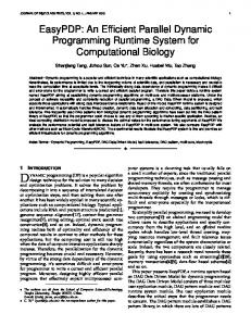
We implement the first-period decisions, update the resources and tasks, and then start the process again at time t + 1. For the deterministic solution, we solve the T period problem using a single expectation of the future. By an expectation, we mean a single demand sample that uses an integer value of the Poisson mean at each location and time period using randomized rounding. For example, if a pair of locations has a mean of 1.3 tasks during a given period, then a particular expectation outcome will have either one task (with probability 0.7) or two tasks (with probability 0.3). The purpose of the randomized rounding is to create an integer data set that is “closer” to the mean than a wider distribution Poisson sample. Since the expectation has single period time windows, it can be solved as a deterministic network that yields an integer optimal solution under that future expectation. This approach is the best that one could ever do using a deterministic technique with an unknown future because the expectation comes from the same Poisson parameters that govern 0 and the solution technique provides integer optimal solutions. The remaining question is estimating the penalty for using the expectation (which is known) instead of 0 (which is not known). For the stochastic training we solve the T -period problem using the multistage CAVE methodology with a different Poisson sample at each iteration. For repeatability, we pregenerated and stored 200 random outcomes from which we sampled at each iteration. For objectivity, 0 was not among the training samples. In the previous deterministic experiments, Transportation Science/Vol. 36, No. 1, February 2002

Percentage of Optimal Posterior Bound

Table 8

98% 96% 94% 92% 90% 88% 86% 84%

Deterministic

82%

Stoch CAVE

80% 0

5

10

15

20

25

30

Horizon Length (4 hour periods)

Figure 8

Rolling-Horizon Comparison of Deterministic Solution and Stochastic Training with 40 Locations and 200 Resources

CAVE produced near-optimal solutions for pure network problems. However, we concluded that the near optimality was due in part to the task state being fixed. Under resampling, the task state changes every iteration, independent of the sequence of decisions and value approximation updates, making the value estimation more difficult. For each combination of number of resources and locations, we perform stochastic and deterministic runs over the 180-period simulation. An optimal posterior bound is calculated by solving the entire simulation under the outcome 0 as a deterministic network. This posterior bound is used to scale the results of the simulations. We undertook a series of experiments to determine an appropriate planning horizon. Figure 8 is typical of these experiments, showing the rolling-horizon results as a function of planning-horizon length for 40 locations and 200 resources. We concluded from these experiments that a 15-period planning horizon was “safe.” Table 9 summarizes the rolling-horizon results for the 15-period planning-horizon length. Using CAVE while resampling provides, on average, a 7% advantage (increasing dramatically as the number of locations increases) over solving a deterministic network problem using the expectation. In general, the CAVE solutions are halfway between the deterministic solution and the posterior bound. The CAVE advantage lies primarily with the superior repositioning decisions made under resampling. The purpose of repositioning is to move resources to locations with better 37


Table 9

Summary of Rolling-Horizon Results with a 15-Period Planning Horizon Using Deterministic and Stochastic Training Percentage of Posterior Bound

No. of Locations

No. of Resources

Deterministic (Expectation) (%)

Stochastic Using CAVE (%)

20 20 20 40 40 40 80 80 80

100 200 400 100 200 400 100 200 400

92.2 96.3 96.6 81.0 90.7 92.6 66.3 81.4 84.8

96.3 97.8 98.1 90.5 96.2 96.8 82.1 93.3 94.5

future opportunities. However, if the future develops differently than expected, little benefit is gained from these movements. If resources are scarce, then the penalty is twofold: There is the wasted repositioning cost and the opportunity cost of the wrong decision. The gap between resampling and using the expectation increases with the number of locations. Repositioning becomes more of a guessing game as the number of locations increases. Since resampling provides a richer view of the future than a single expectation, guessing under resampling is more likely to lead to better future opportunities. Also, the gap between resampling and using the expectation increases as the fleet size decreases. As before, it is due to the greater consequences of unnecessary repositioning when fewer resources are available.

6.

Conclusions

We have made the following contributions to the solution of stochastic, dynamic resource allocation problems with single period travel times. First, we extended the CAVE methodology of Godfrey and Powell (2001) to solve multistage problems. Second, we showed that the CAVE logic provided consistently high-quality solutions within 0.5%–3% of a relaxed optimal bound on deterministic problems with a variety of resource sizes, repositioning costs, number of locations, and horizon lengths. In those cases where the solution quality was less than 99% of the relaxed bound, we argued that the reason was a combination of an integrality gap due to the relaxed bound 38

(especially when resources are scarce), and the separable approximation of a nonseparable value function (especially as the number of locations increases), and the lack of task information in the approximation that we chose. Third, the CAVE method produces high-quality solutions (95%–99% of the relaxed bound) an order of magnitude or two faster than the competing LAMA method of Carvalho and Powell (2000) with similar final solution quality over a wide range of problems. Finally, we estimated the value of stochastic over deterministic modeling for stochastic problems with an uncertain future at 2%–16% where the realized benefit of CAVE increases as the number of resources decreases or as the number of locations increases. Acknowledgments

This research was supported in part by Grant AFOSR-F49620-93-10098 from the Air Force Office of Scientific Research and by Grant DMI00-85368 from the National Science Foundation.

References

Bertsekas, D., J. Tsitsiklis. 1996. Neuro-Dynamic Programming. Athena Scientific, Belmont, MA. Birge, J. 1985. Decomposition and partitioning techniques for multistage stochastic linear programs. Oper. Res. 33(5) 989–1007. , F. Louveaux. 1997. Introduction to Stochastic Programming. Springer-Verlag, New York. Carvalho, T. A., W. B. Powell. 2000. A multiplier adjustment method for dynamic resource allocation problems. Transportation Sci. 34 150–164. Chen, Z-L., W. Powell. 1999. A convergent cutting-plane and partial-sampling algorithm for multistage linear programs with recourse. J. Optim. Theory Appl. 103(3) 497–524. Cheung, R. K-M., W. B. Powell. 1996. An algorithm for multistage dynamic networks with random arc capacities, with an application to dynamic fleet management. Oper. Res. 44(6) 951–963. , . 2000. SHAPE: A stochastic hybrid approximation procedure for two-stage stochastic programs. Oper. Res. 48(1) 73–79. Culioli, J-C., G. Cohen. 1990. Decomposition/coordination algorithms in stochastic optimization. SIAM J. Control Optim. 28 1372–1403. Dantzig, G. 1955. Linear programming under uncertainty. Management Sci. 1 197–206. Ermoliev, Y. 1988. Stochastic quasigradient methods. Y. Ermoliev, R. Wets, eds. Numerical Techniques for Stochastic Optimization. Springer-Verlag, Berlin, Germany. Frantzeskakis, L., W. B. Powell. 1990. A successive linear approximation procedure for stochastic dynamic vehicle allocation problems. Transportation Sci. 24(1) 40–57.



Godfrey, G. A., W. B. Powell. 2001. An adaptive, distributionfree approximation for the newsvendor problem with censored demands, with applications to inventory and distribution problems. Management Sci. 48(8) 1101–1112. , . 2002. An adaptive, dynamic programming algorithm for dynamic fleet management, II: Multiperiod travel times. Transportation Sci. 36(1). Higle, J., S. Sen. 1991. Stochastic decomposition: An algorithm for two stage linear programs with recourse. Math. Oper. Res. 16(3) 650–669. Infanger, G. 1994. Planning Under Uncertainty: Solving Large-scale Stochastic Linear Programs. The Scientific Press Series, Boyd & Fraser, New York. Jordan, W., M. Turnquist. 1983. A stochastic dynamic network model for railroad car distribution. Transportation Sci. 17 123–145. Kall, P., S. Wallace. 1994. Stochastic Programming. John Wiley and Sons, New York. Pereira, M., L. Pinto. 1991. Multistage stochastic optimization applied to energy planning. Math. Programming 52 359–375. Powell, W. B. 1986. A stochastic model of the dynamic vehicle allocation problem. Transportation Sci. 20 117–129. . 1987. An operational planning model for the dynamic vehicle allocation problem with uncertain demands. Transportation Res. 21B 217–232.

. 1989. A review of sensitivity results for linear networks and a new approximation to reduce the effects of degeneracy. Transportation Sci. 23(4) 231–243. , T. A. Carvalho. 1998. Dynamic control of logistics queueing network for large-scale fleet management. Transportation Sci. 32(2) 90–109. , J. A. Shapiro, H. P. Simão. 2002. A representational paradigm for dynamic resource transformation problems. R. Fourer, C. Coullard, J. Owens, eds. Ann. Oper. Res. J. C. Baltzer AG. Forthcoming. Puterman, M. L. 1994. Markov Decision Processes. John Wiley and Sons, New York. Rockafellar, R. T. 1972. Convex Analysis, 2nd ed. Princeton University Press, Princeton, NJ. , R. Wets. 1991. Scenarios and policy aggregation in optimization under uncertainty. Math. Oper. Res. 16(1) 119–147. Ruszczynski, A. 1980. Feasible direction methods for stochastic programming problems. Math. Programming 19 220–229. . 1987. A linearization method for nonsmooth stochastic programming problems. Math. Oper. Res. 12(1) 32–49. Sutton, R., A. Barto. 1998. Reinforcement Learning. The MIT Press, Cambridge, MA. Van Slyke, R., R. Wets. 1969. L-shaped linear programs with applications to optimal control and stochastic programming. SIAM J. Appl. Math. 17(4) 638–663.

Received: December 2000; revision received: August 2001; accepted: September 2001.


39