A Fast Algorithm for Finding Crosswalks using ... - Semantic Scholar

A Fast Algorithm for Finding Crosswalks using Figure-Ground Segmentation James M. Coughlan and Huiying Shen Smith-Kettlewell Eye Research Institute San Francisco, CA 94115 USA {coughlan, shen}@ski.org

Abstract. Urban intersections are the most dangerous parts of a blind person’s travel. Proper alignment is necessary to enter the crosswalk in the right direction and avoid the danger of straying outside the crosswalk. Computer vision is a natural tool for providing such alignment information. However, little work has been done on algorithms for finding crosswalks for the blind, and most of it focuses on fairly clean, simple images in which the Hough transform suffices for extracting the borders of the crosswalk stripes. In real-world conditions such as cluttered scenes with shadows, saturation effects, slightly curved stripes and occlusions, the Hough transform is often unreliable as a pre-processing step. We demonstrate a novel, alternative approach for finding zebra (i.e. multiplely striped) crosswalks that is fast (just a few seconds per image) and robust. The approach is based on figure-ground segmentation, which we cast in a graphical model framework for grouping geometric features into a coherent structure. We show promising experimental results on an image database photographed by an unguided blind pedestrian, demonstrating the feasibility of the approach.

2

1

Introduction

Urban intersections are the most dangerous parts of a blind person’s travel. While most blind pedestrians have little difficulty walking to intersections using standard orientation and mobility skills, it is very difficult for them to align themselves precisely with the crosswalk. Proper alignment would allow them order to enter the crosswalk in the right direction and avoid the danger of straying outside the crosswalk. Little work has been done on algorithms for detecting zebra crosswalks for the blind and visually impaired [10, 4, 5, 9]. This body of work focuses on fairly simple images in which the Hough transform is typically sufficient for extracting the borders of the crosswalk stripes. However, in real-world conditions, such as cluttered scenes with shadows, saturation effects, slightly curved stripes and occlusions, the Hough transform is often inadequate as a pre-processing step. Instead of relying on a tool for grouping structures globally such as the Hough transform, we use a more flexible, local grouping process based on figure-ground segmentation (or segregation) using graphical models. Figure-ground segmentation has recently been successfully applied [8, 3] to the detection and segmentation of specific objects or structures of interest from the background. Standard techniques such as deformable templates [12] are poorly suited to finding some targets, such as printed text, stripe patterns, vegetation or buildings, particularly when the targets are regular or texturelike structures with widely varying extent, shape and scale. The cost of making the deformable template flexible enough to handle such variations in structure and size is the need for many parameters to estimate, which imposes a heavy computational burden. In these cases it seems more appropriate to group target features into a common foreground class, rather than seek a detailed correspondence between a prototype and the target in the image, as is typically done with deformable template and shape matching techniques. Our graphical model-based approach to figure-ground segmentation emphasizes the use of the geometric relationships of features extracted from an image as a means of grouping the target features into the foreground. In contrast with related MRF techniques [2] for classifying image pixels into small numbers of categories, our approach seeks to make maximal use of geometric, rather than intensity-based, information. Geometric information is generally more intuitive to understand than filter-based feature information, and it may also be more appropriate when lighting conditions are highly variable. We formulate our approach in a general figure-ground segmentation framework and apply it to the problem of finding zebra crosswalks in urban scenes. Our results demonstrate a high success rate of crosswalk detections on typical images taken by an unguided blind photographer.

2

Graphical Model for Figure-Ground

We tackle the figure-ground segmentation problem using a graphical model that assigns a label of figure or ground to each element in an image. In our application

3

the elements are a sparse set of geometric features created by grouping together simpler features in a greedy, bottom-up fashion. The features are designed to occur commonly on the foreground structure of interest and more rarely in the background. For example, in our crosswalk application, simple edges are grouped into candidate crosswalk stripe fragment features, i.e. edge pairs that are likely to border fragments of the crosswalk stripes. The true positive features tend to cluster into regular structures (roughly parallel stripes in this case), differently from the false positives, which are distributed more randomly. Our approach exploits this characteristic clustering of true positive features, drawing on ideas from work on object-specific figure-ground segmentation [8], which uses normalized cuts to perform grouping. We use affinity functions to measure the compatibilities of pairs of elements as potential foreground candidates and construct a graphical model to represent a figure-ground process. Each node in the graph has two possible states, figure or ground. The graphical model defines a probability distribution on all possible combinations of figureground labels at each node. We use belief propagation (BP) to estimate the marginal probabilities of these labels at each node; any node with a sufficiently high marginal probability of belonging to the figure is designated as figure. 2.1

The Form of the Graphical Model

We define the graphical model for a general figure-ground segmentation process as follows. Each of the N features extracted from the image is associated with a graph node (vertex) xi , where i ranges from 1 through N . Each node xi can be in two possible states, 0 or 1, representing ground and figure, respectively. The probability of any labeling QN of all the Q nodes is given by the following expression: P (x1 , . . . , xN ) = 1/Z i=1 ψi (xi ) ψij (xi , xj ). (Here we adopt the notation commonly used in the graphical model literature [11], in which the word “potential” corresponds to a factor in this expression for probability. This is different from to the usage in statistical physics, in which potentials must be exponentiated to express a factor in the probability, e.g. e−Ui where Ui is a potential.) This is the expression for a pairwise MRF (graphical model), where ψi (xi ) is the unary potential function, ψij (xi , xj ) is the binary potential function and Z is the normalization factor. < ij > denotes the set of all pairs of features i and j that are directly connected in the graph. ψi (xi ) represents a unary factor reflecting the likelihood of feature xi belonging to the figure or ground, independent of the context of other nearby features. ψij (xi , xj ) is the compatibility function between features i and j, which reflects how the relationship between two features influences the probability of assigning them to figure/ground. The unary and binary functions may be chosen by trial and error, as in the current application, or by maximum likelihood learning. An example of this kind of learning is in [6], in which compatibilities (binary potentials) learned from labeled data are used to construct graphical models for clustering. However, for the preliminary results we show to demonstrate the feasibility of our approach, we used simple trial and error to choose unary and binary functions.

4

The general form of our unary and binary functions is as follows. First, ψi (xi ) enforces a bias in favor of each node being assigned to the ground: ψi (xi = 0) = 1 (which we refer to as a “neutral” value for a potential) and ψi (xi = 1) < 1. The magnitude of the figure value for any feature will depend on one or more unary cues, or factors. In order for a node to be set to the foreground, the binary functions must reward compatible pairs of nodes sufficiently to offset the unary bias. Ground-ground and ground-figure interactions are set to be neutral: ψij (xi = 0, xj = 0) = ψij (xi = 0, xj = 1) = ψij (xi = 1, xj = 0) = 1. Figure-figure interactions ψij (xi = 1, xj = 1) are set less than 1 for relatively incompatible nodes and greater than 1 for compatible nodes. The value of ψij (xi = 1, xj = 1) will be determined by several binary cues, or compatibility factors.

3

Figure-Ground Process for Finding Lines

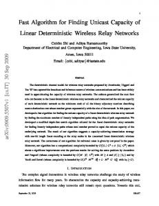
A standard approach to detecting crosswalk stripes is to use the Hough transform to find the straight-line edges of the stripes, and then to group them into an entire zebra pattern. While this method is sound for analyzing high-quality photographs of sufficiently well-formed crosswalks, it is inadequate under many real-world conditions because the Hough transform fails to isolate the lines correctly. To illustrate the limitations of the Hough transform, consider Figure 1. A straight line is specified in Hough space as a pair (d, θ): this defines a line made up of all points (u, v) such that n(θ)·(u, v) = d, where n(θ) = (cos θ, sin θ) is the unit normal vector to the line. In an image containing one straight line, each point of the line will cast votes in Hough space, and collectively the votes will concentrate on the true value of (d, θ). The lines in Figure 1 are not perfectly straight, however, and so the peak in Hough space corresponding to each line will be smeared. If only one such line were present in the image, this smearing could be tolerated simply by quantizing the Hough space bins coarsely enough. However, the presence of a second nearby line makes it difficult for the Hough transform to resolve the two lines separately, since no choice of Hough bin quantization can group all the votes from one line without also including votes from the other.

Fig. 1. Two slightly curved lines (black), representing edges of crosswalk stripes (with exaggerated curvature). The straight red dashed line is tangent to both lines, which means that the Hough transform cannot resolve the two black lines separately.

The global property of the Hough transform is inappropriate for such situations, which is why we turn to a local figure-ground process instead.

5

3.1

Local Figure-Ground Process

Our local figure-ground process is a graphical model with a suitable choice of unary and binary potentials. Given oriented edgelets yi = (Ei , di , θi ) where Ei is the edge strength, di = ui cos θi +vi sin θi and (ui , vi ) are the pixel coordinates of the point, we can define the unary potential as ψi (xi ) = e(αEi +β)xi where α and β are coefficients that can be learned from training data. With this defintion, note that ψi (xi ) always equals 1 whenever xi = 0, and that ψi (xi = 1) increases with increasing edge strength (assuming α > 0). Similarly, we can define the binary potential as ψij (xi , xj ) = e(λCij +τ )xi xj where Cij = |di −dj |+sin2 (θi −θj ) measures how collinear edgelets yi and yj are. Again, note that ψij (xi , xj ) always equals 1 whenever at least one of the states xi , xj is 0. Unless the graph has very dense connectivity, with edgelets being connected even at very long separations, the grouping of edgelets may lack long-range coherence. Without such long-range coherence, the graph may group edgelets into lines that are very slowly curving everywhere (e.g. a large circle) rather than just finding lines that are globally roughly straight. However, such dense connectivity creates great computational complexity in running BP to perform inference. The solution we adopt to this problem is to create a much smaller (and thus faster), higher-scale version of the original graph based on composite feature nodes, each composed of many individual features. For our line grouping problem, we propose a greedy procedure to group the edgelets into roughly straight-line segments of varying length. We describe how this framework applies to crosswalk detection in the next section.

4

Crosswalks and Stripelets

We have devised a bottom-up procedure for grouping edges into composite features that are characteristic of zebra crosswalks, and which are uncommon elsewhere in street scenes. The image is converted to grayscale, downsampled (by a factor of 4 with our current camera) to the size 409x307 and blurred slightly. We have avoided the use of color since we wish to detect crosswalks of arbitrary color. Since the crosswalk stripes are roughly horizontal under typical viewing conditions, our edge detector finds roughly horizontal edges by finding local minima/maxima of a simple y derivative of the image intensity, ∂I/∂y. A greedy procedure groups these individual edges into roughly straight line segments (see Figure 3(a)). A candidate stripe fragment feature, or “stripelet,” is defined as the composition of any two line segments (referred to as “upper” and “lower”) with all of the following properties: (1.) The upper and lower segments have polarities consistent with a crosswalk stripe, i.e. ∂I/∂y is negative on the upper segment and positive on the lower segment, since the crosswalk stripe is painted a much brighter color than the pavement. (2.) The two segments are roughly parallel

6

in the image. (3.) The segments have sufficient “overlap,” i.e. the x-coordinate range of one segment has significant overlap with the x-coordinate range of the other. (4.) The vertical width w of the segment pair (i.e. the y-coordinate of the upper segment minus the y-coordinate of the lower, minimized across x belonging to both segments) must be within the range 2 to 70 pixels (i.e. spanning the typical range of stripe widths observed in our 409x307 images). Many stripelets are detected in a typical crosswalk scene (see Figure 3(b)). 4.1

Crosswalk Graphical Model

Once the stripelets (i.e. nodes) of the graph have been extracted, unary and binary cues are used to evaluate their suitability as “figure” elements. The unary cue exploits the fact that stripes lower in the image tend to be wider, which is true assuming that the camera is pointed rightside-up so that the stripes lower in the image are closer to the photographer. If we examine the empirical distribution of all stripelets (not just the ones that lie on the crosswalks) extracted from our image dataset, we find a characteristic relationship between the vertical widths w and vertical coordinates y (i.e. the vertical height of the centroid of the stripelet in the image). Figure 2 shows a typical scatterplot of (y, w) values from stripelets extracted from a single crosswalk image. The envelope of points in the lower left portion of the graph, drawn as a red line, corresponds to the distribution of stripelets that lie on the crosswalk. The slope and intercept of the envelope will vary depending on the crosswalk, camera pose and presence of non-crosswalk clutter, but typically few points lie left of the envelope. In general, the closer a point is to the envelope, the more likely it is to correspond to a stripelet lying on the crosswalk. Given a crosswalk image, a line-fitting procedure can be used to estimate the envelope, and thereby provide unary evidence for each stripelet belonging to figure (crosswalk) or ground. Let E denote the distance (in (y, w) space) between a (y, w) point and the envelope, and w ˆ be the value of w along the envelope corresponding to the vertical coordinate y of the stripelet. Then E/w ˆ is a normalized measure of distance from the envelope. Another source of unary evidence is the length of the stripelet: all else being equal, long (i.e. horizontally extended) stripelets are more likely to belong to figure than to ground. Denoting the lengths of the upper and lower segments of a stripelet by a and b, we choose a measure L that is the square root of the geometric mean of a and b: L = (ab)1/4 . We combine these two sources of unary evidence into the unary function as follows: ψi (xi = 1) = (1/10) max[1, L(1 − E/w)]. ˆ Longer stripelets that lie close to the envelope will have larger values of unary potential for figure, ψi (xi = 1), but note that this value never exceeds 1/10, compared to the unary potential for ground, 1. One binary cue is applied in two different ways to define the binary potential between two stripelets. This cue is based on the cross ratio test [1] (the application of which is inspired by crosswalk detection work of [10, 9]), which is

7

Fig. 2. Typical scatterplot of (y, w) values from stripelets extracted from single crosswalk image. Envelope of points, drawn as a red line, corresponds to distribution of stripelets lying on the crosswalk.

a quantity defined for four collinear points (in 3-D space) that is invariant to perspective projection. The first application of the cross ratio test is used to check for evidence that the four line segments corresponding to the two stripelets are approximately parallel in three-dimensional space, as they should be. The cross ratio is calculated by drawing a “probe” line through the four lines in the image defined by the line segments. If the four lines share a vanishing point (i.e. because they are parallel in 3-D), the cross ratio should be the same no matter the choice of probe. In our algorithm, we choose two vertical probes to estimate the cost ratio twice, i.e. values of r1 and r2 , and the less discrepant these two values, the higher the compatibility factor. In addition, we exploit a geometric property of a zebra crosswalks: the stripe widths are equal to the separation between adjacent stripes (in 3-D), and so the cross ratio from any line slicing across adjacent stripes should equal 1/4, as pointed out by [9]. These two properties of the cross ratio are combined into an overall error measure as follows: R = (|r1 − 1/4| + |r2 − 1/4|)/2 + 2|r1 − r2 |. This in turn is used to define the binary potential ψij (xi = 1, xj = 1) = (10/3)e−10R . 4.2

Crosswalk Implementation and Results

Since the line-fitting procedure for finding the envelope is confused by noisy scatterplots, multiple envelope hypotheses can be considered if necessary, each of which gives rise to a separate version of the graph. In our experiments we chose eight different envelope hypotheses and ran BP on each corresponding graph. The solution that yielded the highest unary belief at any node was chosen as the final solution. For each graph, the graph connectivity was chosen according to three factors describing the relationship between each possible pair of stripelets: distance between the stripe centroids, the cross ratio error measure R, and the “monotonicity” requirement that the higher stripe must have less vertical width than the lower stripe (i.e. the slope of the envelope is negative). If the distance is not

8

too long, the error measure is sufficiently low and the monotonicity requirement is satisfied, then a connection is established between the stripelets. A few sweeps of BP (one sweep is a schedule of asynchronous BP message updating that updates every possible message once) are applied to each graph, and the unary beliefs, i.e. estimates of P (xi = 1), are thresholded to decide if each feature belongs to the figure or ground. The effects of pruning out the “ground” states are shown in Figure 3 and Figure 4. We ran our algorithm with the same exact settings and parameter values for all of the following images. The total execution time was a few seconds per image, using unoptimized Python and C++ code running on a standard laptop. Note the algorithm’s ability to handle considerable amounts of scene clutter, shadows, saturation, etc. Also note that all photographs were taken by a blind photographer, and no photographs that he took were omitted from our zebra crosswalk dataset.

Fig. 3. Stages of crosswalk detection. Left to right: (a) Straight line segments (green). (b) Stripelets (pairs of line segments) shown as red quadrilaterals. (c) Nodes in graphical model. (d) Figure nodes identified after BP.

5

Summary and Conclusions

We have demonstrated a novel graphical model-based figure-ground segmentation approach to finding zebra crosswalks in images intended for eventual use by a blind pedestrian. Our approach is fast (a few seconds per image) as well as robust, which is essential for making it feasible as an application for blind pedestrians. We are currently investigating learning our graphical model parameters from ground truth datasets, as well as the possibility of employing additional cues. We would like to thank Roberto Manduchi for useful feedback. Both authors were supported by the National Institute on Disability and Rehabilitation Research grant number H133G030080 and the National Eye Institute grant number EY015187-01A2.

References 1. R.I. Hartley and A. Zisserman. ”Multiple View Geometry in Computer Vision”. 2000. Cambridge University Press.

9

Fig. 4. Crosswalk detection results for all zebra crosswalk images.

2. X. He, R. S. Zemel and M. A. Carreira-Perpinan. “Multiscale Conditional Random Fields for Image Labeling.” CVPR 2004. 3. S. Kumar and M. Hebert. “Man-Made Structure Detection in Natural Images using a Causal Multiscale Random Field.” CVPR 2003. 4. S. Se. ”Zebra-crossing Detection for the Partially Sighted.” CVPR) 2000. South Carolina, June 2000. 5. S. Se and M. Brady. ”Road Feature Detection and Estimation.” Machine Vision and Applications Journal, Volume 14, Number 3, pages 157-165, July 2003. 6. N. Shental, A. Zomet, T. Hertz and Y. Weiss. “ Pairwise Clustering and Graphical Models.” NIPS 2003. 7. J. Shi and J. Malik. ”Normalized Cuts and Image Segmentation.” IEEE Transactions on Pattern Analysis and Machine Intelligence, 22(8), 888-905, August 2000. 8. S. X. Yu and J. Shi. “Object-Specific Figure-Ground Segregation.” CVPR 2003. 9. M. S. Uddin and T. Shioyama. “Bipolarity- and Projective Invariant-Based ZebraCrossing Detection for the Visually Impaired.” 1st IEEE Workshop on Computer Vision Applications for the Visually Impaired, CVPR 2005.

10 10. S. Utcke. ”Grouping based on Projective Geometry Constraints and Uncertainty.” ICCV ’98. Bombay, India. Jan. 1998. 11. J.S. Yedidia, W.T. Freeman, Y. Weiss. “Bethe Free Energies, Kikuchi Approximations, and Belief Propagation Algorithms”.2001. MERL Cambridge Research Technical Report TR 2001-16. 12. A. L. Yuille, “Deformable Templates for Face Recognition”. Journal of Cognitive Neuroscience. Vol 3, Number 1. 1991.