online social networks), biological networks (protein interactions) have degree distributions that follow a power law, e.g., the fraction of the vertices that have.
A scalable multilevel algorithm for graph clustering and community structure detection Hristo N. Djidjev1
?
Los Alamos National Laboratory, Los Alamos, NM 87545
Abstract. One of the most useful measures of cluster quality is the modularity of the partition, which measures the difference between the number of the edges joining vertices from the same cluster and the expected number of such edges in a random (unstructured) graph. In this paper we show that the problem of finding a partition maximizing the modularity of a given graph G can be reduced to a minimum weighted cut problem on a complete graph with the same vertices as G. We then show that the resulted minimum cut problem can be efficiently solved with existing software for graph partitioning and that our algorithm finds clusterings of a better quality and much faster than the existing clustering algorithms.
1
Introduction
One way to analyze and understand the information contained in the huge amount of data available on the WWW and the relationships between the individual items is to organize them into ”communities,” maximal groups of related items. Determining the communities is of great theoretical and practical importance since they correspond to entities such as collaboration networks, online social networks, scientific publications or news stories on a given topic, related commercial items, etc. Communities also arise in other types of networks such as computer and communication networks (the Internet, ad-hoc networks) and biological networks (protein interaction networks, genetic networks). The problem of identifying communities in a network is usually modeled as a graph clustering (GC) problem, where vertices correspond to individual items and edges describe relationships. Then the communities correspond to clusters with a lot of edges between vertices belonging to the same subgraph (called incluster edges) and fewer edges between vertices from different subgraphs (called between-cluster edges). The GC problem has been intensively studied in the recent years in relation to its applications in the analysis of networks. Girvan and Newman propose in [11], [18] algorithms based on the betweenness of the edges of a graph, a characteristic that measures the number of the shortest paths in a graph that use any given edge. In [15] Newman describes an algorithm based on a characteristic of clustering quality called modularity, a measure that takes ?
This work has been supported by the Department of Energy under contract W-705ENG-36.
into account the number of in-cluster edges and the expected number of such edges. (We formally define and discuss modularity in more detail in the next section.) A faster version of the algorithm from [15] was described by Clauset et al. in [6]. Several algorithms have been proposed based on the eigenvectors of the graph Laplacian, e.g., [19], [16]. In all previous cases the algorithms reported in the literature are either not fast enough, or are inaccurate. In this paper we will describe a new approach for GC that uses our newly discovered relationship between the GC and the minimum weighted cut problems. The minimum weighted cut (MWC) problem is, given a graph G = (V, E) with real weights on its edges, find a partition of V such that the set of all edges of G that join vertices from different sets of the partition, called a cut of the partition, is of minimum weight. GC looks related to the MWC problems since, in a good quality clustering, the weight of the edges between different sets of the partition (the cut) should be small compared to the weight of the edges inside the sets. But the MWC problem can not be directly applied to solve the GC problem since it does not take into account the sizes of the subgraphs induced by the cut (e.g., it is likely that the minimum cut will consist of the edges incident to a single vertex). There are some minimum cut based clustering algorithms, e.g., [9], that use maximum flow computations combined with heuristics, but they are typically slower than modularity based algorithms, e.g. [6], and, moreover, they cannot determine the optimal number of clusters and, instead, construct a hierarchical decomposition of the set of all vertices of the graph. In this paper we prove that the problem of finding a partition of a graph G that maximizes the modularity can be reduced to the problem of finding a MWC of a weighted complete graph on the same set of vertices as G. We then show that the resulting minimum cut problem can be solved by modifying existing fast algorithms for graph partitioning. We demonstrate by experiments that our algorithm has generally a better quality and is much faster than the best existing GC algorithms.
2 2.1
Our clustering algorithm Graph clustering as a minimum cut problem
As there is no formal definition of clustering and what the clusters of a given graph are, in general it is not possible to determine if a certain partition is the ”correct” clustering or which of two alternative partitions of a graph corresponds to a better clustering. For that reason, researchers have used their intuition to define measures for cluster quality that can be used for comparing different partitions of the same graph. One such measure, introduced in [18,17], which has received considerable attention recently, is the modularity of a graph. Given an n-vertex m-edge graph G = (V (G), E(G)) and a partition P of V (G) into k subsets (clusters) V1 , . . . , Vk , the modularity Q(P) of P is a number defined as k
Q(P) =
1 X (|E(Vi )| − Ex(Vi , G)), m i=1
where E(Vi ) is the set of all edges of G with endpoints in Vi and Ex(Vi , G) is the expected number of such edges in a random graph with a vertex set Vi from a given random graph distribution G. Q(P) measures the difference between the number of in-cluster edges and the expected value of that number in a random (e.g., without cluster structure) graph on the same vertex set. Larger values of Q(P) correspond to better clusterings. Having the definition of Q(P), we can formulate the clustering problem as finding a partition P = {V1 ∪ . . . ∪ Vk } of V (G) such that k X
( |E(Vi )| − Ex(Vi , G)) → max .
(1)
i=1
Clearly max{ P
k X
( |E(Vi )| − Ex(Vi , G) )}
i=1
= − min{ − P
k X
( |E(Vi )| − Ex(Vi , G) )}
i=1
= − min{ (|E(G)| − P
k X
|E(Vi )| ) − (|E(G)| −
i=1
k X
Ex(Vi , G) )}
i=1
= − min{ |Cut(P)| − ExCut(P, G)}, P
where Cut(P) is defined as the cut of P and ExCut(P, G) the expected value of Cut(P) for a random graph from G. Hence, instead of problem (1), one can address the problem of finding a partition P of G such that |Cut(P)| − ExCut(P, G) → min .
(2)
The last expression shows that we can solve (1) as a problem of finding a MWC in a complete graph G0 with a vertex set V (G) and weight weight(i, j) on any edge (i, j) ∈ E(G0 ) defined by � 1 − pij , if (i, j) ∈ E(G) weight(i, j) = (3) −pij , if (i, j) 6∈ E(G), where pij is the probability that there is an edge between vertices i and j in a random graph from the class G. Then, problem (1) is equivalent to the problem of finding a partition P 0 of G0 such that |Cut(P 0 )| → min . We summarize these observations in the following theorem.
(4)
Theorem 1. The problem of finding a partition of a given graph G = (V, E) that minimizes the modularity can be reduced in O(|V | + |E|) time to the problem of finding a minimum weight cut in a complete graph G0 = (V, E 0 ) with edge weights given by (3). For the reduction time bound in Theorem 1 we assume that the edges of E 0 \ E are defined implicitly. There are several choices for G that have been favored by various researchers. The random graph model G(n, p) of Erd¨os-Renyi [7] defines n vertices and puts an edge between each pair � with probability p. Clearly, the expected number of edges of G(n, p) is n2 p. Hence, for a graph with expected number of edges m pij = p =
m � · n
(5)
2
One disadvantage of the G(n, p) model is that it fails to capture important features of the real-world networks, in particular, the degree distribution. As has been recently observed [3], many important types of networks like technological networks (the Internet, the WWW), social networks (collaboration networks, online social networks), biological networks (protein interactions) have degree distributions that follow a power law, e.g., the fraction of the vertices that have degree k > 0 is roughly proportional to αk −λ for some constants α and λ > 0. Such networks are called scale-free. In comparison, the degrees of a random graph from the G(n, p) model follow a �Poisson distribution, i.e., the probability that a given vertex has degree k is nk pk (1 − p)n−k and the expected degree of each vertex is pn. Hence, the Erd¨os-Renyi model may not be suitable as a choice for G when used for determining the community structure of graphs of the above type. One model that takes into account the degrees of the vertices is studied by Chung and Lu in [5]. In that model, the probability that there is an edge between a vertex i and a vertex j is di dj pij = Pn k=1
dk
,
(6)
where d1 , · · · , dn are positive Pnreals corresponding to the degrees of the vertices such that max1≤i≤n d2i < i=1 di . (The last condition guarantees that such a graph exists if all numbers di are integers.) We will refer to that model as the Chung-Lu (CL) model. Clearly, in the CL model, the expected degree of vertex i is di , compared with pn (i.e., independent on i) in the G(n, p) model. In the next section we will describe an efficient method for finding a MWC of a graph G0 with weights on the edges satisfying (3) and pij defined by (5) or (6). 2.2
Finding a MWC using multilevel graph partitioning
Above we established an important relationship between the graph clustering and the MWC problems, i.e., that the problem of finding a partition of a given
graph that maximizes the modularity can be reduced to the problem of finding a minimum weight cut. Most existing work on the MWC problem considers the case where all weights are non-negative. The MWC problem in the case of nonnegative weights is known to be polynomially solvable, e.g., by using algorithms for computing maximum flows [1]. In contrast, the MWC problem in case of realvalue weights is NP-hard and there is very little known for the general version of the problem. Here we show that available heuristics for another related problem, graph partitioning, can be adapted to solve this version of the MWC problem. Overview of the multilevel partitioning method. Formally, the graph partitioning (GP) problem is, given a graph G = (V, E), find a partition (V1 , V2 ) of V such that ||V1 | − |V2 || ≤ 1 (i.e., the partition is balanced ) and Cut(V1 , V2 ) is minimized. (Some versions of the problem consider partitions of arbitrary cardinalities.) Note that, in comparison with the minimum cut problem, there is the additional requirement for a balanced partition. Because of its important applications, e.g., in high performance computing and VLSI design, GP is a well-researched problem for which very efficient methods have been developed. One such approach is the multilevel GP, which is both fast and accurate for a wide class of graphs that appear in practical applications. Inspired by the multigrid method from computational mathematics, it has been used in the works of Barnard and Simon [4], Hendrickson and Leland [10], Karypis and Kumar [12,13], and others. The method for bisecting a graph consists of the following three phases(Figure 2.2): Coarsening phase. The original graph G is coarsened by partitioning it into connected subgraphs and replacing each of the subgraphs by a single vertex and replacing the set of the edges between any pair of shrunk subgraphs by a single edge. Moreover, a weight of each new vertex (respectively edge) is assigned equal to the sum of the weights of the vertices (respectively edges) that it represents. (Weights on the original vertices of G will be defined depending on whether the G(n, p) or the CL model has been used, as detailed below.) The resulting graph is coarsened repeatedly by the same procedure until one gets a graph of a sufficiently small size. Let G0 = G, G1 , . . . , Gl be the resulting graph sequence. Partitioning phase. The graph Gl is partitioned into two parts using any available partitioning method (e.g., spectral partitioning or the Kernighan-Lin (KL) algorithm [14]). Uncoarsening and refinement phase. The partition of Gl is projected on Gl−1 . Since the weight of each vertex of Gl is a sum of the weights of the corresponding vertices of Gl−1 , then the partition of Gl−1 will be balanced if the partition of Gl is and the cut of both partitions will have the same weight. However, since Gl−1 has more vertices than Gl , it has more degrees of freedom and, therefore, it is possible to refine the partition of Gl−1 in order to reduce its cut size. For this end, the projection of the partition of Gl is followed by a refinement phase, which is usually based on the KL algorithm. In the same way, the resulted partition of Gl−1 is converted into a partition of Gl−2 and refined, and so on until a partition of G0 is found.
se
se ni n
ar
g
Co
Un co
ar
ng ni
Partitioning
Fig. 1. The stages of multilevel partitioning. Kernighan-Lin refinement. Since the refinement step is the most involved part of the algorithm, and which ultimately determines its accuracy and efficiency, we will describe it in more detail. It has been shown [13] that the KL algorithm can be a good choice for performing the refinement. The KL algorithms involves several iterations, each consisting of moving a vertex from one set of the partition to the other. Let P = {P1 , P2 } be the current partition. For each vertex u of the graph a gain for u is defined as X X gain(u) = weight(u, v) − weight(u, v), (7) v∈N (u)\P (u)
v∈N (u)∩P (u)
where N (u) is the set of all neighbors of u and P (u) is that set of P that contains u. gain(u) measures how the weight of the cut will be affected if u is moved from P (u) to the other set of P. The KL algorithm then selects a vertex w from the smaller set of the partition with a maximum gain, moves it to the other set, and updates the gains of the vertices adjacent to w. Moreover, w is marked so that it will not be moved again during that refinement step. The process is continued until either all vertices have been moved, or the 50 most recent moves have not led to a better partition. At the end of the refinement step, the last s ≤ 50 moves that have not improved the partition are reversed. Implementation. The implementation of our algorithm for clustering is based on the version of multilevel partitioning implemented by Karypis and Kumar [12,13], which has been made freely available as a software package under the name METIS. Note that graph partitioning, minimum cut, and clustering are
Problem Clustering Minimum Cut Graph Partitioning Objective Minimize modularity Minimize cut size Minimize cut size Balance of partition Sizes may differ Sizes may differ Equal sizes Cardinality of partition To be computed To be computed An input parameter
Table 1. Comparison between the clustering, minimum cut, and partitioning problems. related, but with important differences problems, as illustrated in Table 1. We already showed how the clustering problem can be reduced to a minimum cut problem and here we will show how the resulting minimum cut problem can be solved by a graph partitioning algorithm based on METIS. Because of the differences between graph partitioning and MWC, we have to make some evident changes. For instance, since graph partitioning requires balanced partitions, we have to drop the requirement for balance of the partition. We have also to determine the cardinality of the partition that minimizes the cut size. But the main implementation difficulty is related to the size of G0 . Although the original graph, G, is typically sparse, i.e., has n� vertices and O(n) edges, the transformed one, G0 , is always dense, as it has n2 = Ω(n2 ) edges. The main challenge will be to construct an algorithm whose complexity is close to linear on the size of the original graph, rather than on the size of the transformed one. We have shown that it is possible to simulate an execution of the multilevel algorithm on G0 by explicitly maintaining information only about the edges from the original graph G and implicitly taking into account the remaining edges by modifying the formulae for computing weights and gains. For instance, if P = {P1 , P2 } is a partition of V (G) and we have computed the value of the cut cut(P1 , P2 ) of G corresponding to P and maintain the values of n1 = |P1 | and n2 = |P2 |, then the cut in G0 corresponding to P is cut(P1 , P2 ) − n1 n2 p in the case of the G(n, p) model and hence can be computed in O(1) time. A similar formula holds for the case of the CL model. Clustering into an optimal number of clusters. The algorithm described above is a bisection algorithm, i.e., it finds a partition (and hence clustering) of the input graph into two parts. Our algorithm for an arbitrary number of clusters uses the following recursive procedure. We run the bisection algorithm described above and let P be the resulting partition. If P consists of only one set (i.e., the original graph G does not have a good cluster partition), we are done. Else, we run recursively the bisection algorithm on the two subgraphs G1 and G2 of G induced by the vertices of the two sets of P. It is important to keep, during that recursive call, the weights of the edges computed during the first iteration instead of recomputing them based on G1 and G2 . The reason is that the random graph model based on G will be different than those based on G1 and G2 since formulae (5) and (6) will produce different values for pij . It
can be proven that, if the bisection algorithm finds a minimum bisection cut, the recursive algorithm described above finds a minimum cut (of any number of parts) and hence finds a clustering maximizing the modularity. Time analysis. By using the analysis of Fiduccia and Mattheyses of the KL algorithm from [8], it follows that clustering any network of n vertices and m edges into two communities by our algorithm takes O(n log n + m) time, where n and m are the numbers of the nodes and links of the network, respectively. Finding a clustering in optimal number of k parts takes O((n log n + m)d) time, where d is the depth of the dendrogram describing the clustering hierarchy. Although the worst-case value of d can be Ω(k), typically d = O(log k) [6].
3
Experiments
We performed a number of experiments on randomly generated graphs in order to measure the accuracy of our algorithm and its efficiency as well as to compare it with previous algorithms. We chose Newman-Girvan algorithm [18] and ClausetNewman-Moore algorithm [6] since they are considered one of the best existing algorithms and because of the code availability. 3.1
Comparison with Newman-Girvan algorithm
Following the experimental setting of [18], we generated random graphs with 128 vertices and 4 communities of size 32 each. The expected degree of any vertex is 16, but the outdegree (the expected number of neighbors of a vertex that belong to a different community) is set to i in the i-th experiment (i ≤ 16). Hence, higher values of i correspond to graphs with weaker cluster structures. The experiment is intended to measure the sensitivity of the algorithm to the quality of clustering. Outdegree Degree Newman-Girvan Ours 1 16 1.00 1.00 2 16 1.00 1.00 3 16 0.98 0.99 4 16 0.97 0.99 5 16 0.95 0.99 6 16 0.85 0.97 7 16 0.60 0.91 8 16 0.30 0.70
Table 2. Comparing the quality of the clustering of our algorithm and [18].
Table 2 compares the quality of the clusterings produced by Newman-Girvan’s algorithm and ours. A clustering produced by any of the algorithms is considered ”correct” if it matches the original partition of communities from the graph
generation phase. (Note that, due to the probabilistic nature of the graphs, the clustering that maximizes the modularity might be different from the original partition, especially if the modularity is low.) Our algorithm classifies correctly more than 99% of the edges for outdegrees 0, 1, 2, 3, 4, 5 and in all cases it is better than Newman-Girvan’s (more than twice better for the case i = 8). 3.2
Comparison with Clauset-Newman-Moore algorithm
Table 3 compares the performance of our algorithm with Clauset, Newman, and Moore’s algorithm [6]. That algorithm has the same quality of the clustering as [15], but is claimed to be much faster. The test graphs in all experiments are random graphs with different number of clusters, sizes, densities, and modularities. Each experiment has been run 100 times on different random graphs. In experiments 1–15 the random graphs were generated in the following way: a graph with no edges is created whose vertices are divided into subsets that correspond to the clusters; then edges are created with probability pin between vertices in the same subset and with probability pout between vertices from different subsets. Experiments 1–8 compare how the performance of the algorithms depends on the number of clusters, which vary from 2 to 9. The results indicate that our algorithm produces always clusterings with better quality, and the difference increases when the number of the clusters grows. In experiments 9–12 the test graphs have the same number of vertices, number of cluster, and modularity, but different densities. Those experiments show that our algorithm is more sensitive when the density decreases, and in all the cases our algorithm performs better. In experiments 13–15, we compare the algorithms when the modularity (the quality of the original clustering) is very low. We determined that with modularity less than approximately 0.15 the algorithm from [6] is better, and if the modularity is greater than 0.15 our algorithm is better. In all the above experiments, the running time of our algorithm is considerably smaller, whereby our algorithm is between 7 and 30 times faster than the algorithm from [6]. Finally, in experiments 16–21 the random graphs were created such that their expected degree sequences satisfy a power law distribution. The exponent of the density function varies from -1.0 in experiment 16 to -2.0 in experiment 21 in increments of -0.2. The results of the experiments imply that in the case of power-law degree distributions (scale-free graphs) the quality of our algorithm consistently beats the one of the algorithm from [6], while our time is in average 54 times smaller than theirs. 3.3
Testing on real-world data graphs
We tested our algorithms on a number of real-world graphs such as the nd.edu domain data [2], the United States college football data [11], and the Zachary’s karate club network [20]. In all cases our algorithm produced clustering consistent with our previous knowledge of the communities. For example, we describe
Exp. # vert. 1 200 2 300 3 400 4 500 5 600 6 700 7 800 8 900 9 200 10 200 11 200 12 200 13 400 14 400 15 400 16 400 17 400 18 400 19 400 20 400 21 400
# edges # clust. 8930 2 14891 3 21853 4 29801 5 38776 6 48706 7 59666 8 71546 9 9932 2 4967 2 2458 2 1238 2 41856 4 43607 4 47797 4 8537 4 4879 4 2653 4 1449 4 888 4 629 4
Qorig QCNM > Qours > .388 0 8 .466 0 22 .474 0 42 .463 0 57 .446 0 70 .426 1 87 .406 2 96 .387 1 99 .298 0 8 .299 0 27 .298 0 50 .295 6 92 .176 32 63 .154 39 60 .122 89 11 .244 0 100 .273 0 100 .308 0 100 .370 0 100 .375 0 100 .394 0 100
Q= 92 78 58 43 30 12 2 0 92 73 50 2 5 1 0 0 0 0 0 0 0
TCNM .61 1.01 1.24 1.71 2.25 2.90 3.71 4.44 .68 .54 .61 .46 1.61 1.66 1.84 1.35 1.33 1.33 1.36 1.35 1.34
Tours .03 .05 .11 .23 .15 .22 .33 .35 .04 .03 .02 .00 .18 .10 .07 .02 .01 .03 .04 .02 .03
Table 3. Comparison between the performances of our algorithm and [6]. Qorig is the modularity of the partition used during graph generation, ”QCNM >”, ”Qours >”, and ”Q =” are the percentages of the cases where the algorithm [6] produced a better modularity, our algorithm produced a better modularity, or both algorithms produced equal modularities, respectively. TCNM and Tours are the times of the algorithm from [6] and ours, respectively.
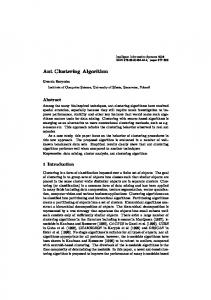
in more detail here the Zachary club network. This example is a standard benchmark for community detection algorithms, describing the interactions between the members of a karate club, which consequently split into two because of between the members, thereby revealing the hidden communities of the original network. As shown on Figure 2, our algorithm classified correctly the members of the two subgroups, except for node 10. That node has the same number of links (five) to both communities, hence adding it to the smaller community results in a greater modularity (e.g., our partitioning has a better modularity than the ”real” one.) 3.4
Measuring the scalability
We also tested the speed of our algorithms by running them on a 2 GHz desktop computer on graphs of different sizes. The results are illustrated on Table 4 and clearly show the extraordinary speed and scalability of our algorithms.
Fig. 2. Zachary’s karate club network. Members of the communities resulting after the split are denoted by circles and squares, respectively. The communities found by our algorithm are separated by the vertical line. pin 0.10 0.14 0.18 0.20 0.20 0.21 0.22
pout 0.01 0.01 0.01 0.011 0.013 0.014 0.015
Vertices 5,000 6,000 7,000 8,000 9,000 10,000 15,000
Edges 406,125 764,126 1,283,398 1,863,710 2,418,730 3,153,106 6,295,801
Total size Time (sec.) 411,125 1.77 770,126 3.09 1,300,398 3.22 1,871,710 6.66 2,427,730 5.68 3,163,106 7.27 6,310,801 15.18
Table 4. Measuring the scalability of our algorithm. pin (respectively pout ) is the expected fraction of the number of in-cluster (respectively between cluster) edges to the number of all pairs of vertices from the same set ( respectively different sets) of the partition used for graph generation.
4
Conclusion
This paper proposes a new approach for graph clustering by reducing the clustering problem to a minimum cut problem and then solving the latter problem by applying methods for graph partitioning. Our proof-of-concept implementation, based on the METIS partitioning package, demonstrated the practicality of the approach. The changes we made to METIS were minimal and various improvements and refinements that take into account the specifics of the clustering problem, use alternative minimum cut or graph partitioning algorithms, or apply heuristics and parameter adjustments in order to improve the accuracy are possible and will be topics of further research.
Acknowledgement. The author is indebted to Melih Onus for helping with the programming and most of the experiments and for many helpful discussions. We also would like to thank the developers of METIS for making their source code publicly available.
References 1. R.K. Ahuja, T.L. Magnanti, J.B. Orlin. Network Flows: Theory, Algorithms, and Applications. Prentice Hall, 1993. 2. R. Albert, H. Jeong and A. L. Barab´ asi. Diameter of the World Wide Web, Nature 401, 130 (1999). 3. A.L. Barab´ asi and R. Albert. Emergence of Scaling in Random Networks. Science 286 (1999), 509-512. 4. S.T. Barnard, H.D. Simon. A fast multilevel implementation of recursive spectral bisection for partitioning unstructured problems. Concurrency: Practice and Experience 6 (1994), pp. 101–107. 5. F. Chung, L. Lu. Connected components in random graphs with given degree sequences. Annals of Combinatorics 6, 125-145 (2002). 6. A. Clauset, M. Newman and C. Moore. Finding community structure in very large networks, Phys. Rev. E 70, 066111 (2004). 7. P. Erdos and A. Renyi. 1959. On random graphs. Publicationes Mathematicae 6:290– 297, 1959. 8. C. M. Fiduccia and R. M. Mattheyses. A linear time heuristic for improving network partitions, IEEE Design Automation Conference, pp. 175-181, 1982. 9. G.W. Flake, R.E. Tarjan, and K. Tsioutsiouliklis. Graph Clustering and Minimum Cut Trees, Internet Mathematics 1:385–408, 2004. 10. B. Hendrickson and R. Leland. A Multilevel Algorithm for Partitioning Graphs, ACM/IEEE conference on Supercomputing, 1995. 11. M. Girvan and M. Newman, Community structure in social and biological networks, Proc. Natl. Acad. Sci. USA 99, 7821–7826, 2002. 12. G. Karypis, V. Kumar. Multilevel graph partitioning schemes, International Conference on Parallel Processing, pp. 113-122, 1995. 13. G. Karypis, V. Kumar. A fast and high quality multilevel scheme for partitioning irregular graphs, SIAM Journal on Scientific Computing, Vol. 20, No. 1, pp. 359392, 1999. 14. Kerninghan B. W. and Lin S. An efficient heuristic procedure for partitioning graphs, The Bell System Technical Journal, 1970. 15. M. Newman, Fast algorithm for detecting community structure in networks, Phys. Rev. E 69, 066133, 2004. 16. M. Newman. Finding community structure in networks using the eigenvectors of matrices, Phys. Rev. E, 74, 036104, 2006. 17. M. Newman. Mixing patterns in networks, Phys. Rev. E 67, 026126, 2003. 18. M. Newman and M. Girvan. Finding and evaluating community structure in networks, Phys. Rev. E 69, 026113, 2004. 19. S. White and P. Smyth. A Spectral Clustering Approach to Finding Communities in Graphs, Proceedings of the SIAM International Conference on Data Mining, 2005. 20. Zachary W. W. An information flow model for conflict and fission in small groups, Journal of Anthropological Research 33, 452-473 (1977).