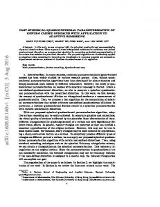
(a) Texture and model. (b) Floater's shape preserving parameterization [6] is used as an initial mesh parameterization. ..... parameterizations of a 3D mesh: a conformal parameter-. 4 .... shop on Rendering 2002, pages 87â98, 2002. [15] P. V. ...
A fast and simple stretch-minimizing mesh parameterization Shin Yoshizawa
Alexander Belyaev
Hans-Peter Seidel
Computer Graphics Group, MPI Informatik, Saarbru¨ cken, Germany Phone: [+49](681)9325-414 Fax: [+49](681)9325-499 E-mails: {shin.yoshizawa | belyaev | hpseidel}@mpi-sb.mpg.de
(a) (b) (c) (d) Figure 1: Texture mapping of the Mannequin Head model with three mesh parameterizations used in our method. (a) Texture and model. (b) Floater’s shape preserving parameterization [6] is used as an initial mesh parameterization. (c) After a single optimization pass. (d) Our optimal low-stretch parameterization.
Abstract
In this paper, we deal with a planar parameterization for a triangle mesh approximating a smooth surface, a bijective mapping between the mesh and a triangulation of a planar polygon. An excellent survey of recent advances in mesh parameterization is given in [7], see also references therein. While various algorithms are developed for mesh parameterization approaches based on solid mathematical theories (e.g., conformal mappings), effective computational schemes for generating practically important low-stretch mesh parameterizations [15] have not yet been proposed. Consider a surface S ∈ R3 topologically equivalent to a disk and given parametrically by r(s, t) = [x(s, t), y(s, t), z(s, t)]. The Jacobian matrix corresponding to the mapping r is given by J = [∂r/∂s, ∂r/∂t, ]. The Jacobian J determines all the first-order geometric properties of the parameterization r(s, t), including the area, angle, and length distortions caused by the mapping r. Denote by Γ(s, t) and γ(s, t) the maximal and minimal singular values of J. Consider the first fundamental form of S:
We propose a fast and simple method for generating a lowstretch mesh parameterization. Given a triangle mesh, we start from the Floater shape preserving parameterization and then improve the parameterization gradually. At each improvement step, we optimize the parameterization generated at the previous step by minimizing a weighted quadratic energy where the weights are chosen in order to minimize the parameterization stretch. This optimization procedure does not generate triangle flips if the boundary of the parameter domain is a convex polygon. Moreover already the first optimization step produces a high-quality mesh parameterization. We compare our parameterization procedure with several state-of-art mesh parameterization methods and demonstrate its speed and high efficiency in parameterizing large and geometrically complex models. Keywords: mesh parameterization, stretch minimization, remeshing
1
Introduction
Surface parameterization consists of a surface decomposition into a set of patches, also referred to as an atlas of charts, and establishing one-to-one mappings between the patches and reference domains. Numerous applications of surface parameterization in computer graphics and geometric modeling include texture mapping, shape morphing, surface reconstruction and repairing, and grid generation.
dl2 = E(s, t)ds2 + 2F (s, t)dsdt + G(s, t)dt2 , where E = r2s , F = rs · rt , and G = r2t . Then Γ2 and γ 2 are the eigenvalues of the metric tensor � � E F JT J = . F G 1
It is convenient to use Γ and γ for measuring various properties of r. For example, if Γ(s, t) = γ(s, t), the parameterization is conformal and mapping r = r(s, t) preserves angles. Since the conformal mappings are well understood mathematically, discrete approximations of conformal mappings are widely used for mesh parameterization purposes [9, 10, 4, 8]. However conformal mappings often produce high stretch regions where texture mappings have severe undersampling artifacts. It is natural p to measure the local stretch of mapping r = r(s, t) by (Γ2 + γ 2 ) /2 [15]. Stretch minimizing mesh parameterizations were considered in [15, 14, 12]. See also [16] where a similar stretch measure is proposed and [11, 19] where the Green-Lagrange tensor is used to measure the stretch. While the stretch minimization approach proposed in [15] and further developed in [14] and [19] leads to generating high-quality mesh parameterizations, the computational procedure used in [15, 14, 19] for stretch minimization is time consuming. Besides the mesh parameterization procedure of [15, 14] often generates regions of high anisotropic stretch, consisting of slim triangles. Such the regions on a parameterized and textured mesh look like cracks and we call them parameter cracks. Fig. 2 demonstrates an appearance of such parameter cracks on the textured Mannequin Head model parametrized by the stretch minimization method from [15].
Parameterization
In this paper, we develop a simple and fast method for generating low-stretch mesh parameterizations. Given a triangle mesh, we first construct the Floater shape preserving mesh parameterization [6]. We improve the parameterization gradually: at each improvement step we optimize the parameterization generated at the previous step. The optimization is achieved by minimizing a weighted quadratic energy with positive weights chosen to minimize the parameterization stretch. Thus the single optimization step is fast since it is based on solving a sparse system of linear equations. Besides if the boundary of the parameterization domain forms a convex polygon, triangle flips never happen [6]. Roughly speaking, our method achieves a low-stretch mesh parameterization via a redistribution (diffusion) of local stretches. It also resembles quasi-Newton type optimization procedures. We compare our low-stretch mesh parameterization procedure with several state-of-art mesh parameterization methods and demonstrate its speed and high efficiency in parameterizing large and geometrically complex models. Besides we show how our mesh parameterization approach can be combined with the interactive geometry remeshing scheme of Alliez et al. [1] in order to achieve fast and high quality remeshing. Fig. 1 shows the three stages of our mesh parameterization method: generating an initial parameterization, our single-pass low-stretch parameterization, and the optimal low-stretch parameterization. The rest or the paper is organized as follows. In Section 2 we explain our low-stretch mesh parameterization procedure and give a motivation behind it. We evaluate our method and compare it with state-of-art mesh parameterization techniques in Section 3. We conclude in Section 4.
Parameter Crack
2 Texture Mapping
Low stretch mesh parameterization
Given a parametrized triangle mesh M ∈ R3 , consider a mesh triangle T = hp1 , p2 , p3 i ∈ M and its corresponding triangle U = hu1 , u2 , u3 i in the parametric plane R2s,t . Triangles {U } define a planar mesh U ∈ R2s,t and the parameterization of M is given by one-to-one mapping between meshes U and M. The correspondence between the vertices of T and U uniquely defines an affine mapping P : U → T . Let us denote by Γ(T ) and γ(T ) the maximal and minimal eigenvalues of the metric tensor induced by the mapping [15, 19]. As we mentioned above, quantity p σ(U ) = (Γ2 + γ 2 ) /2
Figure 2: Parameter cracks on textured Mannequin Head model parametrized by the stretch minimization method of Sander et al. [15].
characterizes the stretch of mapping P . For each vertex ui in the parameter domain let us define its stretch σi = σ(ui ) by r .X X A(Tj )σ(Uj )2 A(Tj ) (1) σi =
In [12] the authors propose to add a regularization term to the stretch energy in order to avoid parameter cracks. The term depends on two parameters. Besides minimizing the resulting energy does not produce a minimal stretch parameterization. 2
h+1 defined by (3) with weights wij
where A(T ) denotes the area of triangle T and the sums are taken over all triangles Tj surrounding mesh vertex pi corresponding to ui . Our method to build a low stretch mesh parameterization consists of several steps. First we construct an initial mesh parameterization using the Floater approach [6]: the boundary vertices of mesh M are mapped into the boundary vertices of U which form a polygon in the parameter plane R2s,t and for each inner vertex pi of M its corresponding vertex ui inside the polygon is selected such that the following local quadratic energy X E(ui ) = wij (uj − ui )2 , (2)
� � h+1 h σ uhj . wij = wij
0 Here wij are the shape preserving weights proposed by Floater. The boundary vertices of the evolving mesh U h , h = 0, 1, 2, . . . , remain fixed. When solving (3) with h+1 numerically we use U h as the initial guess wij = wij for the numerical solver we employ. We use the L2 stretch metric of Sander et al. [15] qX X Esh = Es (U h ) = A(T )σ(U h )2 / A(T ), (5)
j
where the sums are taken over all the triangles T of mesh M, to define a stopping Namely, if Esh+1 ≥ Esh � hcriterion. opt we consider U = ui as an optimal low stretch mesh parameterization. � Besides U opt we also consider U 1 = u1i , the mesh parameterization obtained after one step of our optimization procedure since, according to our experiments, already the first step dramatically improves the parameterization quality. We also can vary the strength of stretch redistribution (diffusion) step (4) by using the weights {σiη }, 0 < η ≤ 1, instead of {σi } in (4): � η old new (6) σj . = wij wij
achieves its minimal value. Here {uj } are vertices corresponding to the mesh one-link neighbors of pi ∈ M and {wij } are positive weights. Now the optimal positions for ui are found by solving a sparse system of linear equations X wij (uj − ui ) = 0. (3) j
This computationally simple procedure produces a valid parameterization of mesh M and avoids triangle flips if the boundary of U is a convex polygon [6]. Now let us estimate local stretch σi = σ(ui ) for each inner vertex ui in the parametric plane. We redistribute the local stretches by assigning � old new = wij wij σj (4)
Using (6) with η < 1 slows down the stretch minimization process but, on the other hand, often improves the mesh parameterization quality. The influence of exponent η in (6) is demonstrated in Fig. 4 for our single-step parameterization U 1 . Choosing smaller values for η leads to a less aggressive stretch minimization. In the next section, we compare U 1 and U opt with results produced by conventional mesh parameterization schemes.
in (2). The new positions of {ui } are now found by solving (3). We can think about vertices {ui } and corresponding energies (2) in terms of a mass-spring system. For an area preserving parameterization, if a high (low) stretch is observed at ui , that is σi > 1 (σi < 1), we relax (strengthen) the springs connected with ui by solving (3) with new weights (4). It works similarly for a general parameterization. Our idea to diffuse the local stretches iteratively by (1), (3), (4) can resemble the relaxation approach of Balmelli et al. [2]. Notice however that in [2] the authors use a gradient-descent minimization approach (an explicit mesh evolution scheme) while our method is similar to quasiNewton type minimization algorithms and an implicit mesh evolution scheme is used. One can also find a similarity between (2), (4) and Winslow’s variable diffusion method [18, 3] for adaptive grid generation (see also [17] for a comprehensive analysis of numerical methods used to minimize Winslow’s variable diffusion functional). We start from the shape � preserving parameterization of Floater [6, § 6] U 0 = u0i and then improve it gradually: � � U h+1 = uh+1 is obtained from U h = uhi by solving i
3
Results and comparisons
Computing. All the examples presented in this section are computed using gcc 2.95 C++ compiler on a 1.7GHz Pentium 4 computer with 512MB RAM. To solve a system of linear equation Ax = b we use PCBCG [13] with the maximum number of iterations equal to 104 and the approximation error |Ax − b| /|b| set to 10−6 .
3
Error metrics. To evaluate the visual quality of a parameterization we use the checkerboard texture shown in the bottom-left image of Fig. 2. For a quantitative evaluation of various mesh parameterization methods we employ L2 stretch metric (5) and consider edge, angle, and area distortion error functions defined below. To measure the edge distortion error we use X |pi − pj | |ui − uj | P |pi − pj | − P |ui − uj | ,
where the sums are taken over all the edges of meshes M and U. The angle distortion error is defined by
Fig. 7 shows U opt parameterization of the Mannequin Head model when the parameter domain has boundaries of various shapes. The left images show the parameterization and corresponding texture mapping results when the boundary is the unit circle. The right images demonstrate similar results when the boundary of the parameter domain was obtained as the so-called natural boundary for the conformal parameterization of [4]. Notice that the stretch distortions near the boundary are substantially reduced in the latter case. In Fig. 8 mesh parameterizations U 0 , U 1 , and U opt are evaluated and compared using the checkerboard texture. Sometimes U opt does not produce the best visual result because of high anisotropy and U 1 is preferable. Finally, in Fig. 9 we analyze how the stretch distribution over a complex geometry model is changing during the optimization process U 0 → U 1 → U opt . The top row of images presents the model (a decimated Max-Planck bust model) and results of checkerboard texture mapping with U 0 , U 1 , and U opt . The four remaining images of the model show the stretch distribution over the model for U 0 , U 1 , and U opt parameterizations. The images demonstrate how well our stretch minimization procedures minimize and equalize the stretch. It is interesting to notice that near the mesh boundary the optimized meshes have large area and angle distortions (the same effect is observed in all the other tested models) but relatively low stretch distortions. One can hope that an appropriate relaxation of boundary conditions will reduce those area and angle distortions while maintaining low stretch.
3 1 XX |θj,i − φj,i | , 3F j i=1
where the sums are taken over all the angles θj,i and φj,i of the triangles of meshes M and U, respectively, and F is the total number of triangles (faces) of M. The area distortion is measured by X X X A (Tj ) − A (Uj ) / A (Uj ) , A (Tj ) /
where the sums are taken over all the triangles of meshes M and U.
Comparison and evaluation. We have implemented a number of conventional mesh parameterization methods and compared them with our low stretch technique: (a) (b) (c) (d) (e) (fh )
Eck et al. harmonic map [5] Floater’s shape preserving parameterization [6, § 6] Desbrun et al. intrinsic parameterization [4] Sander et al. stretch minimizing parameterization [15] Our single-step parameterization U 1 Our optimal parameterization U opt
The subindex h in (fh ) in the bottom row of the above table shows the total number of optimization steps (3), (4) needed to generate U opt . Tables 1-12 and Figures 3 and 6 present qualitative and visual comparisons of the above mesh parameterization schemes tested on various models topologically equivalent to a disk. The unit square is used as the parameter domain and for each models its the boundary vertices are fixed on the boundary of the square. The errors and computational times measured in seconds (s) and sometimes in minutes (m) and hours (h) are given. For the intrinsic parameterization method [4], we use the equal blending of the Dirichlet and Authalic energies for all the models, except for the Fish model (Table 11) where we use only the Dirichlet energy in order to avoid triangle flips. Our single-step mesh parameterization procedure (generating U 1 ) is only slightly slower than the fast Floater and Eck et al. parameterization methods and faster than the intrinsic parameterization of Desbrun et al. [4]. Besides U 1 demonstrates competitive results in minimizing the stretch, edge, area, and angle distortions. Our optimal mesh parameterization procedure is also fast enough and sometimes achieves better results in stretch minimizing than the probabilistic minimization of Sander et al. [15] which is very slow. Moreover, by contrast with [15], U opt does not generate parameter cracks (see Fig. 6) because (3) acts like a diffusion process. Besides, if a very low stretch parameterization is needed, U opt can be used as an initial parameterization for [15].
Application to remeshing. In the right column of Fig. 3 and in Fig. 5 we demonstrate how our mesh parameterization technique can be used for fast and high quality remeshing of complex surfaces. We have chosen the interactive geometry remeshing scheme of Alliez et al. [1] and implemented its main steps: 1. Create a mesh parameterization. 2. Compute area, curvature, and control maps using hardware accelerated OpenGL commands. 3. Sample points by applying an error diffusion to the control map. 4. Connect the points using the Delaunay triangulation. 5. Use the parameterization to map the points into 3D. A conformal mesh parameterization is the best choice for the described remeshing scheme. It is clear that the remeshing quality depends on the size of an image used for the hardware assisted acceleration: the bigger size, the better result. On the other side, the image size is restricted by the graphics card memory. It turns out that a high quality remeshing can be obtained even for a relatively small image size. Let us assume that we have two parameterizations of a 3D mesh: a conformal parameter4
Acknowledgments
ization and an area-preserving one. Then let us the areapreserving parameterization for computing the control map and resampling the points via an error diffusion process. Finally, the points are mapped from the area-preserving parameterization to the conformal one and are connected using the Delaunay triangulation. The above remeshing modification has one drawback: it requires two parameterizations, conformal and areapreserving. However since our low-stretch parameterization U opt has nice area-preserving properties and the initial Floater’s parameterization U 0 is close to a conformal one, we use U opt and U 0 instead of the conformal and areapreserving parameterizations in the above modification of the interactive geometry remeshing scheme of Alliez et al. Right images (a)-(c) of Fig. 3 demonstrate results of the single-parameterization remeshing scheme if the discrete harmonic map parameterization [5], Floater’s shape preserving parameterization [6], and intrinsic discrete conformal parameterization are used, respectively. Right images (d)-(f) of Fig. 3 present our experiments with the doubleparameterization remeshing scheme. We set Floater’s parameterization U 0 as a substitute of a conformal parameterization and used U 0 as an initial parameterization to generate the stretch-minimizing parameterization of Sander et al. [15] and U 1 and U opt . These low-stretch parameterizations were used as substitutes of an area-preserving parameterization. Fig. 5 presents remeshed Max-Planck bust and Stanford bunny models obtained by�the remeshing � 0 , U 0 , U 1 , and schemes based on (from left to right) U � 0 opt U ,U parameterizations (here using {U 0 , U 00 } parameterizations means that we use U 0 as a substitute of a conformal parameterization and U 00 as a substitute of an area preserving one). Notice�that the double-parameterization remeshing scheme with U 0 , U opt produces the best results.
4
The authors would like to thank Hugues Hoppe for a helpful discussion and the anonymous reviewers of this paper for their valuable and constructive comments. The models are courtesy of the Stanford University (bunny and dragon), the University of Washington (mannequin head and fish), Cyberware Inc. (Igea), and MPI f¨ur Informatik (Max-Planck bust).
References [1] P. Alliez, M. Meyer, and M. Desbrun. Interactive geometry remeshing. In Proceedings of ACM SIGGRAPH 2002, pages 347–354, 2002. [2] L. Balmelli, G. Taubin, and F. Bernardini. Space-optimized texture maps. In Proceedings of EUROGRAPHICS 2002, pages 411–420, 2002. [3] W. Cao, W. Huang, and R. D. Russell. Approaches for generating moving adaptive meshes: location versus velocity. Appl. Numer. Math., 47:121–138, 2003. [4] M. Desbrun, M. Meyer, and P. Alliez. Intrinsic parameterizations of surface meshes. In Proceedings of EUROGRAPHICS 2002, pages 209–218, 2002. [5] M. Eck, T. DeRose, T. Duchamp, H. Hoppe, M. Lounsbery, and W. Stuetzl. Multiresolution analysis of arbitrary meshes. In Proceedings of ACM SIGGRAPH 1995, pages 173–182, 1995. [6] M. S. Floater. Parametrization and smooth approximation of surface triangulations. Computer Aided Geometric Design, 14(3):231–250, 1997. [7] M. S. Floater and K. Hormann. Recent advances in surface parameterization. In Multiresolution in Geometric Modelling, pages 259– 284, 2003. [8] X. Gu and S.-T. Yau. Global conformal surface parameterization. In Proceedings of Eurographics Symposium on Geometry Processing 2003, pages 135–146, 2003. [9] S. Haker, S. Angenent, A. Tannenbaum, R. Kikinis, G. Sapiro, and M. Halle. Conformal surface parameterization for texture mapping. IEEE Transactions on Visualization and Computer Graphics, 6(2):181–189, 2000. [10] B. L´evy, S. Petitjean, N. Ray, and J. Maillot. Least squares conformal maps for automatic texture atlas generations. In Proceedings of ACM SIGGRAPH 2002, pages 362–371, 2002. [11] J. Maillot, H. Yahia, and A. Verroust. Interactive texture mapping. In Proceedings of ACM SIGGRAPH 1993, pages 27–34, 1993. [12] E. Praun and H. Hoppe. Spherical parametrization and remeshing. In Proceedings of ACM SIGGRAPH 2003, pages 340–349, 2003. [13] W. H. Press, S. A. Teukolsky, W. T. Vetterling, and B. P. Flannery. Numerical Recipies in C. Cambridge University Press, 1988. [14] P. V. Sander, S. J. Gortler, J. Snyder, and H. Hoppe. Signalspecialized parametrization. In Proceedings of Eurographics Workshop on Rendering 2002, pages 87–98, 2002. [15] P. V. Sander, J. Snyder, S. J. Gortler, and H. Hoppe. Texture mapping progressive meshes. In Proceedings of ACM SIGGRAPH 2001, pages 409–416, 2001. [16] O. Sorkine, D. Cohen-Or, R. Goldenthal, and D. Lischinski. Bounded-distortion piecewise mesh parameterization. In Proceedings of IEEE Visualization, pages 355–362, 2002. [17] A. M. Winslow. Numerical solution of the quasilinear poisson equation in a nonuniform. J. Comput. Phys., 2:149–172, 1967. [18] A. M. Winslow. Adaptive mesh zoning by equipotential method. Technical report, Lawrence Livermore Laboratory, 1981. Report UCID-19062. [19] E. Zhang, K. Mischaikow, and G. Turk. Feature-based surface parameterization and texture mapping. Technical report, Georgia Institute of Technology, 2003. GVU Tech Report 03-29.
Conclusion
We have presented a fast and powerful method for generating low-stretch mesh parameterizations and demonstrate its applicability to high quality texture mapping and remeshing. Our method is much faster than the stochastic stretch minimization procedure of Sander et al. [15] (note that their more recent coarse-to-fine stretch optimization procedure [14] is significantly faster than that of [15] but still slower than ours) and often produces better quality results. In particular, it does not generate parameter cracks. Our method is heuristic. At present we are not able to support it by rigorous mathematical results. In future we plan to extend our approach to spherical parameterizations and use quadratic energies with matrix weights for incorporating an anisotropy in our optimization process. 5
PARAMETERIZATION C URVATURE M AP
(a) Harmonic map of Eck et al. [5]:
T EXTURE M APPING
time 0.37 s,
(b) Floater shape preserving weights [6]:
time 0.32 s,
(c) Intrinsic parameterization of Desbrun et al. [4]:
(d) Stretch minimization of Sander et al. [15]:
(e) Our U 1 parameterization:
(f) Our U opt = U 3 parameterization:
Stretch: 6.661,
time 0.5 s,
time 1.09 s,
Edge: 0.997,
Stretch: 5.792,
time 0.76 s,
time 23 m,
PARAMETER C RACKS ?
Edge: 0.959, Angle: 0.18,
Stretch: 6.129,
Stretch: 1.327,
Stretch: 1.642,
Stretch: 1.382,
Angle: 0.068,
Edge: 0.978,
Edge: 0.539,
Edge: 0.507,
Edge: 0.4748,
Area: 1.403
Area: 1.373
Angle: 0.12,
Angle: 0.274,
Angle: 0.383,
R EMESHING [1]
Area: 1.388
Area: 0.495
Area: 0.871
Angle: 0.4132,
Area: 0.3832
Figure 3: Comparison of various mesh parameterization schemes on the Mannequin Head model (V = 2732, F = 5420).
6
time 0.06 s 0.06 s 0.12 s 80.91 s 0.08 s 0.16 s
(a) (b) (c) (d) (e) (f3 )
Stretch 6.6507 5.9171 6.2751 1.375 1.6691 1.4084
Edge 0.9918 0.9635 0.9778 0.5162 0.5084 0.4814
Angle 0.125 0.1995 0.1619 0.2952 0.3717 0.4479
Area 1.4032 1.3801 1.3931 0.5232 0.8836 0.4165
(a) (b) (c) (d) (e) (f8 )
Table 1: Mannequin Head model: V = 689, F = 1355
(a) (b) (c) (d) (e=f1 )
time 0.21 s 0.17 s 0.33 s 213 s 0.3 s
Stretch 1.9708 1.8084 1.8511 1.172 1.2057
Edge 0.4935 0.4648 0.4753 0.2996 0.2862
Angle 0.0969 0.1568 0.1189 0.2239 0.2881
(a) (b) (c) (d) (e) (f3 )
Stretch 6.6617 5.7921 6.1295 1.3279 1.6425 1.382
Edge 0.9971 0.9599 0.9784 0.5393 0.5073 0.4748
Angle 0.0685 0.1807 0.1209 0.2744 0.3838 0.4132
Area 0.8455 0.8409 0.84 0.3043 0.3179
(a) (b) (c) (d) (e) (f3 )
(a) (b) (c) (d) (e) (f3 )
Stretch 13.306 11.729 12.266 1.3408 1.7643 1.4791
Edge 0.7563 0.6976 0.7232 0.4955 0.4551 0.4661
Angle 0.1041 0.2545 0.176 0.3477 0.3735 0.5226
(a) (b) (c) (d) (e) (f2 )
(a) (b) (c) (d) (e) (f3 )
Stretch 18.027 15.941 16.933 1.3257 2.2037 1.5392
Edge 1.2288 1.2074 1.2157 0.7021 0.6249 0.5623
Angle 0.0361 0.1441 0.0857 0.2501 0.372 0.4905
(a) (b) (c) (d) (e) (f6 )
(a) (b) (c) (d) (e) (f3 )
Stretch 1.5348 1.485 43.947 1.2226 1.2105 1.1718
Edge 0.3025 0.3412 0.7602 0.2833 0.2477 0.24
Angle 0.1313 0.1748 0.3622 0.1934 0.2112 0.2636
Area 1.7599 1.7175 1.7387 0.8435 1.4739 0.7897
time 12.4 s 8.95 s 90.7 s 43.4 h 14.7 s 32.3 s
Stretch 9462.1 181.05 320.53 1.6816 3.3929 2.884
Edge 0.9729 0.9983 0.9845 0.7193 0.5041 0.6399
Angle 0.0704 0.3852 0.2281 0.2917 0.6184 0.7747
Area 1.5132 1.5725 1.5425 0.6665 0.8078 0.5344
time 11.2 s 8.46 s 93.8 s 18.6 h 15.2 s 27.2 s
Stretch 3.4799 4.676 34.621 1.3092 1.4373 1.304
Edge 0.7924 0.8678 0.8104 0.4603 0.4166 0.385
Angle 0.0542 0.1627 0.1831 0.2265 0.3446 0.3923
Area 1.3399 1.3664 1.3525 0.5492 0.6868 0.4123
time 17.9 s 13.2 s 231 s 55.6 h 22.5 s 79.8 s
Stretch 712.33 85.181 672.45 1.5159 4.7926 1.8755
Edge 0.7097 0.7241 0.7062 0.4982 0.4582 0.6143
Angle 0.0797 0.1522 0.2866 0.3109 0.387 0.6065
Area 1.098 1.0861 1.0957 0.4868 0.5632 0.5241
Table 10: Stanford Bunny model: V = 31272, F = 62247
Area 1.692 1.6373 1.6618 0.5436 1.1899 0.6217
(a) (b) (c0 ) (d) (e) (f2 )
Table 5: Decimated Max-Planck bust model: V = 9462, F = 18866
time 12.9 s 6.21 s 25.8 s 4.5 h 17.9 s 42.6 s
Angle 0.0915 0.3491 0.2707 0.3544 0.6341 0.8253
Table 9: Igea model: V = 24720, F = 49301
Area 1.0207 0.9526 0.9795 0.4227 0.4676 0.3613
Table 4: Cat model: V = 5649, F = 11168
time 3.16 s 2.29 s 17.4 s 57.5h 4.18 s 9.22 s
Edge 1.6037 1.5049 1.5494 1.1442 0.9883 0.8522
Table 8: Dragon Head model: V = 23929, F = 47783
Area 1.4036 1.3733 1.3886 0.4956 0.8717 0.3832
Table 3: Refined Mannequin Head model: V = 2732, F = 5420
time 1.23 s 0.87 s 1.81 s 1h 1.5 s 3.44 s
Stretch 9179549 1120318 231989 7635.3 313.64 3.5688
Table 7: Half-of-Dragon model: V = 13927, F = 27782
Table 2: Cat Head model: V = 1856, F = 3660
time 0.37 s 0.32 s 0.76 s 23 m 0.5 s 1.09 s
time 5.55 s 4.24 s 21.1 s 39.7 h 6.99 s 33.2 s
time 92.4 s 66.3 s 486 s 120 h 125 s 206 s
Stretch 6.3061 6.092 6.306 2.5689 1.5683 1.5041
Edge 0.8241 0.7752 0.8241 0.6481 0.4252 0.4414
Angle 0.0445 0.1782 0.0445 0.2444 0.3476 0.4678
Area 1.3021 1.2613 1.3021 0.926 0.6387 0.3946
Table 11: Fish model: V = 64982, F = 129664
Area 0.5063 0.5651 1.0085 0.4338 0.3876 0.2375
(a) (b) (c) (e) (f3 )
Table 6: Fandisk model: V = 9919, F = 19617
time 250 s 204 s 52.1 m 384 s 848 s
Stretch 18.207 18.1025 2.8434 2.2094 1.4926
Edge 1.2578 1.25 1.2341 0.6598 0.5939
Angle 0.03 0.0512 0.3068 0.3698 0.4865
Area 1.6936 1.6912 1.6924 1.2017 0.4812
Table 12: Max-Planck bust model: V = 199169, F = 398043
7
Figure 4: Choosing smaller values for η leads to a less aggressive stretch minimization. From left to right: U 1 parameterization of Mannequin Head with η = {0, 0.1, 0.2, 0.4, 0.6, 0.8, 1}.
Figure 5: Remeshing of Max-Planck (three left images) and Stanford bunny (three right images) models. For each model � bust model � remeshings according to U 0 , U 0 , U 1 , and U 0 , U opt are shown. See the text for details.
Figure 6: Parameter cracks on various models textured with checkerboard texture. The images of the upper row demonstrate parameter cracks generated by the stretch-minimization method of Sander et al. [15]. The images of the bottom row show the same parts of the models parameterized by our U opt .
U opt = U 5 with circular parameter domain. Time: 1.51 s, Stretch: 1.34, Edge: 0.43, Angle: 0.47, Area: 0.4.
U opt = U 1 with natural boundary [4]. Time:1.67 s, Stretch: 1.68, Edge: 0.5, Angle: 0.37, Area: 0.9.
Figure 7: Using various parameter domains for U opt .
8
U0
U1
Ave:11.12
Min:0.17
U1
Min:0.21
Max:37.96
U opt
Ave:2.11
Max:4.51
Figure 9: Top row: a decimated Max-Planck bust model and results of checkerboard texture mapping with U 0 , U 1 , and U opt parameterizations. The four remaining images of the model show the distribution of the vertex stretches over the model for U 0 , U 1 , and U opt . Firstly coloring by stretch σ ∈ [0.17, 37.96] is used to compare U 0 and U 1 . Then the same coloring scheme on the stretch interval [0.21, 4.51] is employed to compare the stretch distributions for U 1 , and U opt . Here the bounds of the interval are equal to the maximal and minimal stretch values.
Figure 8: Checkerboard texture mapping with U 0 (left), U 1 (middle), and U opt (right).
9