Aug 2, 2013 - s.t. tr{CiZ} + 1 ⤠0, âi = 1,2,3; Z â½ 0. (3). Notations: Boldface uppercase and lower case letters denote matrices and vectors respectively.
1
A Fast Eigen Solution for Homogeneous Quadratic Minimization with at most Three arXiv:1308.0104v1 [math.NA] 1 Aug 2013
Constraints Dinesh Dileep Gaurav, Student Member, IEEE and K.V.S. Hari, Senior Member, IEEE
Abstract We propose an eigenvalue based technique to solve the Homogeneous Quadratic Constrained Quadratic Programming problem (HQCQP) with at most 3 constraints which arise in many signal processing problems. Semi-Definite Relaxation (SDR) is the only known approach and is computationally intensive. We study the performance of the proposed fast eigen approach through simulations in the context of MIMO relays and show that the solution converges to the solution obtained using the SDR approach with significant reduction in complexity. Index Terms Homogeneous Quadratic Minimization, Semi-Definite Relaxation, MIMO Relay.
I. I NTRODUCTION Fast Algorithms for non-convex Homogeneous Quadratic Constrained Quadratic Programming (HQCQP) are much sought after as many important problems in wireless communications and signal processing can be formulated as HQCQP problems. In [1], the authors solve a physical layer multi-casting problem where an M antenna transmitter is transmitting the same data to K single antenna receivers which was formulated as a HQCQP problem with N = M 2 variables and K constraints. In [2], the authors consider the design of optimal relay precoding
matrix for an N -antenna Multiple-Input Multiple-Output (MIMO) relay which minimizes the relay power Dinesh Dileep Gaurav and K.V.S. Hari are with SSP Lab, Department of Electrical Communication Engineering, Indian Institute of Science, Bangalore 560012, India (e-mail: {dileep, hari}@ece.iisc.ernet.in). The financial support of the DST, India and of the EPSRC, UK under the auspices of the India-UK Advanced Technology Centre (IU-ATC) is gratefully acknowledged. August 2, 2013
DRAFT
2
while satisfying constraints on Signal-to-Interference-plus-Noise Ratio (SINR) at the M receivers. It is shown that this is a HQCQP with N 2 variables and M constraints. Also in [3], a multi-user multi-relay peer-to-peer beamforming problem is considered, which can be reformulated as a HQCQP. In [?], [?], relay power minimization problems are considered in the context of two-way MIMO relaying which can be reformulated as a HQCQP. In addition, HQCQP problems arise naturally when one applies alternating optimization techniques to several transmit precoder design problems [4] and in robust beamforming [5]. Semi-Definite Relaxation (SDR) has become a dominant tool to solve HQCQP in recent years [6] but is computationally expensive. In this letter, we address the HQCQP problem with two and three constraints separately. Our main contributions are (a) proving that the non-convex HQCQP can be solved by solving an equivalent Eigen Value Problem (EVP) which is convex (b) and that the EVP can be solved using iterative techniques like search methods leading to significant reduction in computational complexity. II. P ROBLEM S TATEMENT We consider the optimization problem [6] min
xH Tx
x ǫ CN ×1
s.t. xH Pi x + 1 ≤ 0, ∀i = 1, 2, 3
(1)
where T ≻ 0 and all Pi are indefinite Hermitian matrices, and x is the N × 1 complex vector to be found. This quadratic optimization problem is referred to as homogeneous as it does not have a linear term in the complex vector x. Using the Cholesky decomposition of T , and letting z = T1/2 x and Ci = T−1/2 Pi T−1/2 , we can rewrite (1) as min zH z, s.t. zH Ci z + 1 ≤ 0, ∀i = 1, 2, 3
(2)
z ǫ CN ×1
Note that the objective function is convex but the constraints are not. III. S EMI -D EFINITE R ELAXATION The only known tractable approach to (2) which is globally convergent is Semi-Definite Relaxation[see [6] and reference therein]. To solve (2), the semi-definite problem min
Z∈CN 2 ×N 2
tr{Z}
s.t. tr{Ci Z} + 1 ≤ 0, ∀i = 1, 2, 3; Z � 0
(3)
Notations: Boldface uppercase and lower case letters denote matrices and vectors respectively. AH , kAkF , tr{A}, A−1 denotes conjugate transpose, frobenius norm, matrix trace, inverse respectively. A � 0 denotes A is positive semi-definite. August 2, 2013
DRAFT
3
is solved. Then one extracts the complex solution vector z from Z using several techniques as explained in [6]. IV. E IGEN A PPROACH In this section, we propose a novel solution for (2) which can be obtained by solving an eigenvalue problem. For reasons of clarity, we present the two-constraints and the three-constraints cases separately (one-constraint case is trivial). A. Two-Constraints Case Consider the polar decomposition of z =
√ pu for a positive scalar p and a unit-norm N × 1 vector
u. Rewriting (2) as p⋆ =
min
p,u,||u||2=1
p, s.t. pci (u) + 1 ≤ 0, i = 1, 2.
(4)
where we define ci (u) = uH Ci u. Note that (4) is feasible only if there exists some u 6= 0 such that ci (u) < 0.
Theorem IV.1. Consider the optimization problem c⋆ =
min
u,||u||2 =1
max (c1 (u), c2 (u)) .
(5)
If uopt is the solution for (5), then it will also be the solution for (4) and p⋆ = −1/c⋆ . Proof: Let u⋆p be the optimum solution for (4) and let u⋆c be the same for (5). Observe that u⋆p will be a feasible solution for (5) with objective value1 −1/p⋆ . Similarly, u⋆c will be a feasible solution for
(4) with corresponding optimum as −1/c⋆ . Let p⋆c = −1/c⋆ . Thus, we need to prove p⋆ = p⋆c . Assume p⋆ < p⋆c . Thus, (−1/p⋆ ) < c⋆ which implies u⋆p leads to a lower objective value for (5) than u⋆c , which
is a contradiction. Now, for the other direction, assume p⋆ > p⋆c . Clearly, u⋆c leads to a lower objective value for (4) than u⋆c which is a contradiction. Thus p⋆ = p⋆c = (−1/c⋆ ). It is interesting to note that each ci (u) is a mapping from the unit sphere U = {u | uH u = 1} to a closed continuous interval on the real line. The endpoints of this interval are given by the minimum and 1
It is easy to see that at least one of the constraints in (4) should be binding (strictly equal) at the optimum. This is because,
if it is not the case, we can decrease p further till one of the constraints becomes equal, thereby decreasing the objective value which is a contradiction.
August 2, 2013
DRAFT
4
maximum eigenvalues of Ci . The interval is the well known "Numerical Range" of a Hermitian matrix [7]. Define the two dimensional set S2 (u) = {[c1 (u), c2 (u)] ∈ R2 | uH u = 1}
(6)
The set S2 (u) is defined as the joint numerical range of Hermitian matrices C1 and C2 [7]. It follows from the Toeplitz-Hausdorff theorem [7] that S2 (u) is a closed compact convex subset of the 2-D plane. Note that only for diagonal matrices, this will be a solid rectangle and for other matrices, it will be any closed compact convex shape in general (see appendix A for an example). Thus, we can interpret (5) as minimizing the convex function max(x, y) over a 2-D convex set S2 (u). It can be shown that the solution of (5) over S2 (u) can occur only at one of the three points in S2 (u), the left-most point on the vertical edge, or the bottom-most point on the horizontal edge, or the extreme bottom-left point which lies on the line c1 (u) = c2 (u)(see appendix B). Let xi denote the unit eigenvector corresponding to λmin (Ci ). Then, by definition, ci (xi ) = λmin (Ci ). Thus (λmin (C1 ), c2 (x1 )) will be the left-most point of S2 and (c1 (x2 ), λmin (C2 )) will be the bottom-most point of S2 . See appendix D for a detailed discussion on
the same and the proof on properties of the max(x, y) function. We state that ⋆ H Case 1: if xH 1 C1 x1 > x1 C2 x1 , then c = λmin (C1 ) and u = x1 . Intuitively, this is the bottom most
point of the 2-D set S2 (u). H ⋆ Case 2: if xH 2 C2 x2 > x2 C1 x2 , , then c = λmin (C2 ) and u = x2 . Intuitively, this is the left most
point of the S2 (u). H H H Case 3: if xH 1 C1 x1 ≤ x1 C2 x1 and x2 C2 x2 ≤ x2 C1 x2 then at the optimal point, c1 (u) = c2 (u).
Defining A1 = C1 and A2 = C1 − C2 , (4) is equivalent to c⋆ =
min
u,uH u=1
uH A1 u,
s.t. uH A2 u = 0.
(7)
This corresponds to finding the bottom-left point of S2 (u) along the diagonal c1 = c2 , [c1 , c2 ] ∈ S2 (u). Case 1 and Case 2 are equivalent to solving for the minimum eigenvalue of a given Hermitian matrix. In these cases, one of the constraints will not be binding (strict inequality). In Case 3, we still need to solve an optimization problem. In the following lemma, we prove it is a semi-definite optimization (SDP) problem. Theorem IV.2. The optimization problem in (7) is equivalent to the following max-min eigenvalue problem. c⋆ = max λ, s.t. (A1 + tA2 ) − λI � 0 λ,t ǫ R
August 2, 2013
(8)
DRAFT
5
Proof: Consider the minimum eigenvalue of A1 + tA2 , λ(t) = min{uH (A1 + tA2 )u | uH u = 1}.
(9)
By adding one more constraint on the RHS, we have λ(t) ≤ min{uH A1 u | uH A2 u = 0, uH u = 1}
(10)
Note that the optimization on RHS is same as (7). We now show that max λ(t) = min{uH A1 u | uH A2 u = 0, uH u = 1}.
t ∈ R
(11)
We prove this by contradiction. Suppose that it is not true and there is strict inequality in (11) and that the maximum value of λ(t) is achieved at t∗ . Consider the set U = {u | uH u = 1, λ(t∗ ) = uH A1 u + t∗ uH A2 u}
(12)
If uH A2 u > 0 for all u ∈ U , then there exist λ(t∗ + ǫ) > λ(t∗ ) for some ǫ > 0, which is a contradiction. Similarly, if uH A2 u < 0 for all u ∈ U , then there exist λ(t∗ − ǫ) > λ(t∗ ) for some ǫ > 0, which is
also a contradiction. If there exists u such that uH A2 u = 0, then (11) should also hold, which is also a contradiction. Thus U contains some vector v with vA2 v > 0 and some vector w with wA2 w < 0. Then some linear combination u of v and w is in U and has uH A2 u = 0. Thus, (11) should be true. Thus, we need to maximize the minimum eigenvalue of A1 + tA2 over all t. Now, for any Hermitian matrix A , minimum eigenvalue is given by the semi-definite program [6]. λmin (A) = max λ, A − λI � 0. λ ǫ R
(13)
Using A = A1 + tA2 in (13) gives the optimization problem in (4) and hence the proof. 1 Once the solution is obtained in (8), we have p = ⋆ and u as the eigenvector corresponding to the |c | minimum eigenvalue of A1 + t⋆ A2 where t⋆ is the optimal value of t from solving (8). It is worth mentioning that (5) has been stated in this form when u is two dimensional and solved using a different approach in [8] in the context of Two-way MIMO Relaying. Our approach can be seen as generalizing it for arbitrary dimension. B. Three-Constraints Case Now we solve the three-constraints case in a similar manner to the two-constraints case. min p, s.t. pci (u) + 1 ≤ 0, i = 1, 2, 3 p,u
August 2, 2013
(14)
DRAFT
6
Following the same arguments as in two-constraints case, solving (14) is equivalent to the optimization problem c⋆ = min H
u u=1
max (c1 (u), c2 (u), c3 (u)) .
(15)
As earlier, we define the set S3 (u) = {[c1 (u), c2 (u), c3 (u)] ∈ R3 | uH u = 1}
(16)
But here, Toeplitz-Hausdorff theorem has to be applied with an exception. S3 (u) is convex for all values of N ≥ 3, but not for N = 2 [7]. Thus, in this paper, we consider all values of N ≥ 3. Unlike the two-constraint case, the minimum of the max function in 3-dimensions is more involved. At the optimum, at least one of the three constraints must be strictly binding, which gives us the three following cases. Case 1: In this case, at the optimum value, all three constraints are binding. Thus, the solution will be lying on the line c1 (u) = c2 (u) = c3 (u). Note that, there is only one such point. Defining A1 = C1 , A2 = C1 − C2 and A3 = C1 − C3 , this is equivalent to solving the optimization problem, c⋆ = min u H A1 u H u u=1
s.t. uH A2 u = 0,
uH A3 u = 0.
(17)
Using the same arguments as in the proof for theorem IV.2, we can prove (17) is equivalent to the semi-definite optimization problem c⋆ =
max
λ,t1 ,t2 ǫ R
λ,
(A1 + t1 A2 + t2 A3 ) − λI � 0
(18)
Case 2: In this case, any two of the constraints will be binding at the optimum. Note that there are three such points in S3 (u). Without loss of generality, assume the first and second constraint will be binding at the optimum. Thus, we have c1 (u) = c2 (u) at the optimum. Then, defining A1 = C1 and A2 = C1 − C2 , we have c⋆ = min uH A1 u, H u u=1
uH A2 u = 0
(19)
Note that we converted the same problem into a SDP problem in lemma IV.2. Thus we can apply those results here to rewrite it as in (8). Case 3: In this case, only one of the constraints will be binding at optimum. Note that there are three such possibilites. It can be shown that if ith constraint is binding, then c⋆ = λmin (Ci ). In the three-constraints case, we are required to find all the seven 3-dimensional points in S3 (u), corresponding to each of this above mentioned cases. After evaluating the cost function at these seven August 2, 2013
DRAFT
7
points, the minimum value yields c⋆ . In numerical examples, we show through extensive simulations that this is still significantly faster than SDR even though it has to solve 4 different optimization problems corresponding to case 1 and case 2. V. I TERATIVE A LGORITHMS In this section, we present iterative algorithms to solve two semi-definite optimization problems in (8) and in (18). Note that, they could also be solved with a convex package. Let M0 , M1 and M2 be N × N Hermitian matrices. We consider the optimization problems max
λ,t1 ǫ R
λ, s.t. (M0 + t1 M1 ) − λI � 0
(20)
and max
λ,t1 ,t2 ǫ R
λ, s.t. (M0 + t1 M1 + t2 M2 ) − λI � 0.
(21)
Optimization problem in (20) is required to solve the case 3 in two-constraints case, and Case 2 in three-constraints case. Similarly, the one in (21) is needed to solve the Case 1 in three-constraints case. We observe that both the problems are concave in the variables. To be specific, we are maximizing the following concave functions λ(t1 ) = λmin (M0 + t1 M1 ) , t1 ∈ R
(22)
λ(t1 , t2 ) = λmin (M0 + t1 M1 + t2 M2 ) , (t1 , t2 ) ∈ R2 ,
(23)
and
respectively. Note that these come under the well known problem of maximizing the minimum eigenvalue of a linear combination of Hermitian matrices which is known to be a convex optimization problem [9]. Thus, to solve (20), any standard one dimensional-search can be used. Similarly, to solve (21), we propose an alternating optimization approach by fixing one variable and optimizing over the other. Since this is a convex optimization problem, it is globally convergent. It is worth mentioning that we could resort to advanced optimization techniques which might improve the speed of convergence rather than simple search methods. But, search methods are attractive since they are efficient to implement in practice. We implement a standard dichotomous search [10] with the initial search interval as [λmin (M0 ), 0] in both the cases. We scaled the interval size whenever |λmin (M0 )| is very large, to accelerate the convergence. It is interesting to note that the majority of computation in each iteration of both problems comes from the minimum eigenvalue calculation. August 2, 2013
DRAFT
8 Relative Error v/s No. of Iterations 1 N=3, N=4, N=5, N=3, N=4, N=5,
0.9
Relative Error − − −− >
0.8
3 3 3 2 2 2
Users Users Users Users Users Users
0.7 0.6 0.5 0.4 0.3 0.2 0.1 0
0
5
10
15
No. of Iterations − − −− >
Fig. 1.
MIMO Relay scenario: Relative Error, ǫi as a function of number of iterations for 2-users and 3-users cases with
varying number of antennas (M ) at the relay.
VI. S IMULATIONS For the purpose of simulation, we consider a practical application to compare SDR and the proposed technique. We consider the MIMO Relay Precoder design problem solved in [2] which minimizes the total relay power subject to SINR constraints at the receivers which is shown to be a HQCQP with number of constraints equal to the number of users, and number of variables is equal to the square of number of antennas. Thus, the proposed technique can be used in the 2-user and the 3-user scenarios. For both the scenarios, we randomly generate 1000 standard complex Gaussian MIMO channels corresponding to M ∈ {3, 4, 5} where M denotes the number of antennas at the Relay. Thus, there are N = M 2 variables in the correspoding HQCQP. The noise variances at all nodes are fixed to be −10 dB and SINR requirement to be 3 dB in all scenarios. Interested reader is urged to refer [2] for a detailed system model and thorough theoretical analysis. Numerical simulations are used to compare two different aspects of the proposed technique when compared against SDR. For solving SDR, we used CVX, a package for solving convex programs [11]. In the first set of simulations, we look at the Average Relative Error of the proposed technique in approaching the true objective value at the optimum which will be obtained from SDR. For the proposed technique, we define the Relative Error ǫi (n) in the ith iteration for the nth problem data as ǫi (n) = |
p⋆ (n) − pˆi (n) | p⋆ (n)
(24)
where p⋆ (n) denotes the true value obtained from SDR and pˆi (n) is the value obtained from the current
August 2, 2013
DRAFT
9
TABLE I MIMO R ELAY SCENARIO : R ATIO OF CPU TIME REQUIRED FOR SDR BASED METHOD TO PROPOSED E IGEN BASED METHOD FOR
2- USERS AND 3- USERS CASE WITH VARYING NUMBER OF ANTENNAS , M .
M =3
M =4
M =5
2 Users
720
304
127
3 Users
54
26
16
iteration of the proposed technique for the nth data set. The Average Relative Error for a particular iteration is then calculated over 1000 such datasets by averaging the Relative Error. Average Relative Error gives an idea of how fast the algorithm converges to the true value in terms of number of iterations. Fig.VI shows the relative error performance of the proposed technique for the 2-constraints (2 users) case and 3-constraints (3-users) case. It is observed that for various N being considered, the proposed technique reaches 90% of the true value in 8-10 iterations. In another set of simulations, we compare the raw CPU times of both SDR and the proposed technique on a standard Desktop PC configuration. The stopping criterion for the dichotomous search in the proposed algorithm is based on a threshold value of 10−4 for the final interval size, while the SDR algorithm uses an internal threshold value for convergence [11]. TABLE I presents a comparison of CPU times for different scenarios. Each entry inside the table specifies the ratio of CPU time based on SDR algorithm and the CPU time based on the proposed algorithm. For instance, for the 2-users case and having 3 antennas, the proposed technique is 720 times faster than SDR based solution. We can see that as the number of antennas increases, the ratio decreases. This can be considered to be due to the limitation of the dichotomous algorithm and also the increase in computational cost of evaluating eigenvalues of a larger matrix. For the 3-users case, the ratio is significantly reduced due to the nature of the cost function and solving multiple eigenvalue problems (compared to the 2-users case). However, the improvement is still significant. Overall, there is significant improvement in the reduction of complexity of the HQCQP minimization problem. VII. C ONCLUSION In this paper, we propose an eigen-framework to solve HQCQP with at most three constraints. We propose iterative techniques which have significant reduction in complexity to solve the same. We demonstrate the benefits using a MIMO relay power minimization problem.
August 2, 2013
DRAFT
10
A PPENDIX A A N I NTRODUCTION
TO J OINT
N UMERICAL R ANGE
OF
H ERMITIAN M ATRICES
Let C1, C2 , . . . , Cm be N × N Hermitian matrices. Define ci (u) = uH Ci u for any unit-norm vector
u for a given i ∈ {1, . . . , m}. Note that ci (u) is always real. Then the set of points in Rm defined as
Sm = { [c1 (u), c2 (u), . . . , cm (u)] ∈ Rm , uH u = 1}
(25)
is defined as the joint numerical range of Hermitian matrices C1 , C2 , . . . , Cm . When m = 1, this reduces to the well-known Rayleigh ratio of a Hermitian matrix which varies from λmin (C1 ) ≤ ci (u) ≤
λmax (C1 ) continuously over the unit sphere uH u = 1 [12]. When m = 2, it becomes a 2 − D set.
From the well known Toeplitz-Hausdorff Theorem [7], it follows that S2 is a closed compact convex set. We provide some pictorial examples for the same. Let N = 4 and m = 2. We consider two randomly generated hermitian matrices C1 , C2 and generate the corresponding S2 . 0.6487 0.4814 − 0.9681i −0.9725 − 1.0067i 0.4814 + 0.9681i −0.2919 0.0625 + 1.0729i C1 = −0.9725 + 1.0067i 0.0625 − 1.0729i −2.1321 −0.5501 + 0.8097i −0.4020 − 0.2913i 0.4457 + 0.4558i 0.8810 1.0909 − 0.2062i −0.3353 + 0.3102i 1.0909 + 0.2062i −0.6045 −0.4007 − 0.0412i C2 = −0.3353 − 0.3102i −0.4007 + 0.0412i −0.4677 −0.1632 + 0.8746i −0.1488 − 0.5651i 0.3299 − 1.0372i
−0.5501 − 0.8097i
−0.4020 + 0.2913i 0.4457 − 0.4558i −1.4286 −0.1632 − 0.8746i −0.1488 + 0.5651i 0.3299 + 1.0372i 0.3086
(26)
(27)
The joint numerical range for the above C1 , C2 is given in Fig:A The greyed solid region in Fig:A shows the 2-D joint numerical range of given hermitian matrices C1 and C2 . This clearly shows that it is not rectangular. It is straightforward to see that the Joint Numerical Range in 2-D will be a solid rectangle if the matrices are diagonal. A PPENDIX B S OME D EFINITIONS Consider any 2 − D closed compact and convex set S2 . We define the following points in this set •
Left-Most Point: We define the left-most point of set S2 as the point whose co-ordinates (xw , yw ) are given by xl = min
(x,y)∈S2
August 2, 2013
x,
yl =
min
(xl ,y)∈S2
y
(28)
DRAFT
11
5
� � Plotting 2-D set S2 = { uH C1 u, uH C2 u ∈ R2 , uH u = 1}
4
3
λmax (C1 ), λmax (C2 )
2
�
1
S2
0
−1
−2
λmin (C1 ), λmin (C2 )
�
−3
−4
−5 −8
−6
−4
−2
0
2
4
6
8
Intuitively, This is the point which lies on the bottom on the left most vertical edge. Note that the
y − axis − − >
left-most vertical edge can be a single point or multiple points.
(xw , yw )
S2
x − axis − − >
(xbl , ybl ) (xb , yb )
Fig. 2.
Demonstration of Defined Points Left-Most, Bottom-Most and Bottom-Left Most points
August 2, 2013
DRAFT
12
•
Bottom-Most Point: We define the bottom-most point of set S2 as the point whose co-ordinates (xs , ys ) are given by yb = min
(x,y)∈S2
y,
xb =
min
(x,yb )∈S2
x
(29)
Intuitively, This is the point which lies on the left-most end on the bottom-most horizontal edge. •
Bottom-Left-Most Point: We define the bottom-left-most point of set S2 as the point whose coordinates (xbl , ybl ) are given by xbl =
min
(x,y)∈S2 ,x=y
x,
ybl = xbl
(30)
Intuitively, this point lies on the lowest end of the line x = y towards the bottom left side . In Fig:B, we give an example of all the three points for a given convex set which in this case is a circular disk. A PPENDIX C B OTTOM -M OST, L EFT-M OST
AND
B OTTOM -L EFT M OST
POINT FOR
S2
Let xi denote the eigenvector corresponding to λmin (Ci ). Thus by definition, ci (xi ) = xH i Ci x = λmin (Ci )
. In S2 , the x − axis corresponds to the numerical range of C1 which ranges from λmin (C1 ) ≤ c1 (u) ≤ λmax (C1 ). Similarly, the y − axis range will be λmin (C2 ) ≤ c2 (u) ≤ λmax (C2 ). Thus, the bottom-
most would correspond to (c1 (x2 ), λmin (C2 )) where c1 (x2 ) = xH 2 C2 x2 . The Bottom-Left point will
correspond to extreme bottom point lying on line x = y i.e. c1 (u) = c2 (u). It can be obtained by solving the problem min c1 (u), c1 (u) = c2 (u)
||u||2 =1
(31)
We consider a circular disk shape in Fig:C to explain this points. We have marked the Bottom-Most, Left-Most and the Bottom-Left Most point in the given shape corresponding to the joint numerical range of the given two hermitian matrices. A PPENDIX D max F UNCTION OVER A CONVEX 2-D SET
We define the max function as max(x, y) =
x, y,
August 2, 2013
if x ≥ y
(32)
if x < y.
DRAFT
y − axis − − >
13
[λmin (C1 ), c2 (x1 )]
S2
x − axis − − >
[c1 (u), c2 (u)] [c1 (x2 ), λmin (C2 )]
Fig. 3.
Demonstration of Defined Points Left-Most, Bottom-Most and Bottom-Left Most points for the Joint Numerical
Range
Thus, at a point (x, y), calculating the function max(x, y) amounts to calculating the maximum value among its two arguments. It is easy to see that max is indeed a convex function from the definition of convex functions itself. We consider the problem of finding the global optimum (x⋆ , y ⋆ ) ∈ S2 of the problem c⋆ = min max (x, y) (x,y)∈S2
(33)
Theorem D.1. Consider the max function over a given 2D closed, compact, convex set S2 . Let us assume the points (xb , yb ) Bottom-Most Point, (xl , yl ) Left-Most Point and (xbl , ybl ) Bottom-Left-Most Point are given for the set S2 . Then 1) The global optimum of the minimum of max function over the convex set S2 will be achieved at one of the points among the Left-Most (xl , yl ) , Bottom-Most (xb , yb ), Bottom-Left most point (xbl , ybl ) of the convex set S2 . 2) Moreover, we have the alternative a) Either if xl > yl , then c⋆ = xl b) or if yb > xb , then c⋆ = yb August 2, 2013
DRAFT
14
c) or if yl > xl and yb < xb , then c⋆ = xbl Proof: 1) Suppose (a, b) is a global minimizer of max(x, y). If a = b, clearly (a, b) must be the bottom left endpoint of the slice of S lying on the line x = y which is the Bottom-Left Most point. Thus c⋆ = xbl in this case.
Now suppose a 6= b. WLOG, assume that a < b (hence max(a, b) = b). Consider the Bottom-Most point (xb , yb ) of the set S2 . We consider the cases •
xb < a. Since yb ≤ b and max(a, b) ≤ max(xb , yb ), we must have yb = b and hence max(a, b) = max(xb , yb ).
•
xb ≥ a. Consider the convex combination (x, y) = (θxb + (1 − θ)a, θyb + (1 − θ)b). This
denotes all the points lying in the line segment between (a, b) and (xb , yb ). Since we have assumed that a < b, we get max(x, y) = θyb + (1 − θ)b when θ is small. In order that this is greater than or equal to b = max(a, b), we must have yb ≥ b. However, by definition of (xb , yb ), this means (a, b) = (xb , yb ).
In a similar line, it is easy to prove that if a > b, then (xl , yl ) is the solution. 2) We prove 2a. Assume xl > yl . From the definition of (xl , yl ) and (xb , yb ), it follows that xl ≤ xb and yb ≤ yl . Then xb > yb (because yb ≤ yl < xl ≤ xb ). Thus max(xl , yl ) = xl ≤ xb = max(xb , yb )
and hence (xl , yl ) should be the optimum.
R EFERENCES [1] N. Sidiropoulos, T. Davidson, and Z.-Q. Luo, “Transmit beamforming for physical-layer multicasting,” IEEE Trans. Signal Process., vol. 54, no. 6, pp. 2239 – 2251, Jun. 2006. [2] B. K. Chalise, L. Vandendorpe, and J. Louveaux, “Mimo relaying for multi-point to multi-point communication in wireless networks,” in 2007 2nd IEEE International Workshop on Computational Advances in Multi-Sensor Adaptive Processing, CAMPSAP, 2007, pp. 217–220. [3] M. Fadel, A. El-Keyi, and A. Sultan, “Qos-constrained multiuser peer-to-peer amplify-and-forward relay beamforming,” IEEE Trans. Signal Process., vol. 60, no. 3, pp. 1397 –1408, Mar. 2012. [4] M. Khandaker and Y. Rong, “Interference mimo relay channel: Joint power control and transceiver-relay beamforming,” IEEE Trans. Signal Process., vol. 60, no. 12, pp. 6509 –6518, Dec. 2012. [5] B. Chalise and L. Vandendorpe, “Optimization of mimo relays for multipoint-to-multipoint communications: Nonrobust and robust designs,” IEEE Trans. Signal Process., vol. 58, no. 12, pp. 6355 –6368, Dec. 2010. [6] Z. quan Luo, W. kin Ma, A.-C. So, Y. Ye, and S. Zhang, “Semidefinite relaxation of quadratic optimization problems,” IEEE Signal Process. Mag., vol. 27, no. 3, pp. 20 –34, May. 2010. August 2, 2013
DRAFT
15
[7] E. Gutkin, E. A. Jonckheere, and M. Karow, “Convexity of the joint numerical range: topological and differential geometric viewpoints,” Linear Algebra and its Applications, 2004. [8] T. M. Kim, B. Bandemer, and A. Paulraj, “Beamforming for network-coded mimo two-way relaying,” in Signals, Systems and Computers (ASILOMAR), 2010 Conference Record of the Forty Fourth Asilomar Conference on, Nov. 2010, pp. 647 –652. [9] L. Vandenberghe and S. Boyd, “Semidefinite programming,” 1996. [10] A. Antoniou and W.-S. Lu, Practical Optimization: Algorithms and Engineering Applications.
Springer, 2007.
[11] I. CVX Research, “CVX: Matlab software for disciplined convex programming, version 2.0 beta,” http://cvxr.com/cvx, Sep. 2012. [12] R. A. Horn and C. R. Johnson, Topics in Matrix Analysis. Cambridge University Press, 1991.
August 2, 2013
DRAFT