merge calls to the same kernels (but operating on different data) into a sin- ... In addition to reducing the call overhead, we gain additional performance by.
A Fast GPU Implementation for Solving Sparse Ill-Posed Linear Equation Systems Florian Stock and Andreas Koch Embedded Systems and Applications Group Technische Universit¨ at Darmstadt {stock|koch}@eis.cs.tu-darmstadt.de
Abstract. Image reconstruction, a very compute-intense process in general, can often be reduced to large linear equation systems represented as sparse under-determined matrices. Solvers for these equation systems (not restricted to image reconstruction) spend most of their time in sparse matrix-vector multiplications (SpMV). In this paper we will present a GPU-accelerated scheme for a Conjugate Gradient (CG) solver, with focus on the SpMV. We will discuss and quantify the optimizations employed to achieve a soft-real time constraint as well as alternative solutions relying on FPGAs, the Cell Broadband Engine, a highly optimized SSE-based software implementation, and other GPU SpMV implementations.
1
Introduction and Problem Description
Modern imaging technologies in many application areas (e.g., medical, security, safety, multi-media) require the efficient solution of large systems of linear equations. In this work, we describe the solution of a practical reconstruction problem under soft-real time constraints as required by an industrial embedded computing use-case. For greater generality, we have abstracted away the individual problem details and concentrate on the solution itself, namely the reconstruction of voxel information from the sensor data. For the specific use-case, this process requires the solution of a matrix system with up to 250 × 106 elements (depending on the image size). However, due to practical limitations of the sensor system (e.g., due to unavoidable mechanical inaccuracies), the gathered data does not allow perfect reconstruction of the original image and leads to a strongly ill-posed linear equation system. To achieve acceptable image quality, a domain-specific regularization, which narrows the solution space, has to be employed. It expresses additional requirements on the solution (such as ∀i : xi ≤ 0) and is applied during each step of the conjugate gradient (CG) method, allowing the reconstruction of suitable-quality images in ≈ 400 CG iterations. It is the need for this regularization vector F as a correction term, that makes other, generally faster equation solving methods (see Section 2) unsuitable for this specific problem. The matrix A, which represents the linear equation system, has up to 855000 nonzero elements. These nonzero elements comprise 0.3 − 0.4% of all elements. If stored as single-precision numbers in a non-sparse manner, it would require more than 2 GB of memory.
ek = AT Adk + F (xk , dk ) fk = dTk ek αk = −(gkT ek )/f k+1 x = xk + αk dk gk+1 = AT (Axk+1 − b) + F (xk , xk+1 ) T βk = (gk+1 ek )/fk dk+1 = −gk+1 + βk dk Table 1. Loop body of the CG algorithm. F is the regularizing correction term.
Multiprocessor Multiprocessor Scalar Processor Multiprocessor Scalar Processor Shared Scalar Processor Scalar Processor Multiprocessor Scalar Processor Shared Scalar Processor Memory Scalar Processor Multiprocessor Scalar Processor Shared Scalar Processor Memory Scalar Processor Scalar Processor Shared Scalar Processor Memory Scalar Processor Scalar Processor Scalar Processor Constant Cache Scalar Processor Texture Cache Shared Scalar Processor Memory Scalar Processor Cache Scalar Processor TextureMemory Cache Constant Scalar Processor Scalar ScalarProcessor Processor Cache Texture Cache Constant Texture Cache Constant Cache Constant Cache Texture Cache
Device Memory
Fig. 1. CUDA architecture
A number of storage formats are available for expressing sparse matrices more compactly (e.g., ELLPACK, CSR, CSC, jagged diagonal format [12]). For our case, as the matrix is generated row-by-row by the sensors, the most suitable approach is the compressed sparse row format (CSR, sometimes also referred as compressed row storage CRS). For our application, this reduces the required storage for A to just 7 MB. As the CG solver demands a positive semi-definite matrix, we use the CGNR (CG Normal Residual) approach [12] and left-multiply the equation system with AT . Hence, we do not solve Ax = b, but AT Ax = b. Due to the higher condition number κ of the matrix AT A, with κ(AT A) = κ(A)2 , this will however result in a slower convergence of the iterative solver. Table 1 shows the pseudo-code for the modified CG algorithm. Computing 400 iterations of this CG (size of matrix A 320,000 × 3,000 with 1,800,000 nonzero entries) requires 15 GFLOPS and a bandwidth of 105 GB/s. The softreal time constraint of the industrial application requires the reconstruction of four different images (taken by different sensors) in 0.44 seconds. However, since these images are independent, they can be computed in parallel, allowing 0.44s for the reconstruction of a single image. The core of this work is the implementation of the modified CG algorithm on a GPU, with a focus on the matrix multiplication. The techniques shown will be applicable to the efficient handling of sparse matrix problems in general. 1.1
GPGPU Computing and the CUDA System
With continued refinement and growing flexibility, graphics processing units (GPUs) can now be applied to general-purpose computing scenarios (GPGPU), often outperforming conventional processors. Nowadays, the architecture of modern GPUs consists of arrays of hundreds of flexible general-purpose processing units supporting threaded computation models and random-access memories. Dedicated languages and programming tools to exploit this many-core paradigm include the manufacturer specific flows CUDA (described below, by NVIDIA) and Firestream [1] by ATI/AMD, as well as the hardware-independent Brook+ [5], RapidMind [9] and OpenCL [6] approaches. For our work, we target NVIDIA GPUs, specifically the GTS 8800 models and GTX 280. They are programmed using the Compute Unified Device Architecture (CUDA) development flow. Figure 1 shows the block diagram of such a CUDAsupported GPU. The computation is done by multiprocessors, which consist
of eight scalar processors, operating in SIMD mode (=all executing the same instruction, but on different data). Each of the scalar processors can execute multiple threads, which it schedules without overhead. This thread scheduling is used to hide memory latencies in each thread. Each multiprocessor furthermore has a small shared memory (16 KB) which is randomly accessible with low latency by all of its scalar processors. The device global memory is also randomly accessible by all scalar processors, but high performance requires that accesses have to occur to sequential addresses. In the threaded model, this implies that consecutive threads must access consecutive memory addresses. Only such accesses, which are called coalesced, allow highbandwidth memory operations, others have a significant performance penalty. An entire computation, a so-called kernel, is instantiated on the GPU device as multiple blocks. These are then executed in arbitrary order, ideally in parallel, but may be serialized, e.g., when the number of blocks exceeds the number of multiprocessors available on the device. The block structure must be chosen carefully by the programmer, since no fast inter-block communication is possible. A block is assigned atomically for execution on a multiprocessor, which then processes the contained threads in parallel in a SIMD manner. Note that the threads within a block may communicate quickly via the shared memory and can be efficiently synchronized. At invocation time, a kernel is parametrized with the number of blocks it should execute in as well as the number of threads within each block (see [10] for more details). For high performance computing (HPC) applications the number of threads is usually much larger than the number of multiprocessors.
2
Related Work
A large number of methods can be used for solving linear equations. They are often classified into different types of algorithms, such as direct methods (e.g., LU decomposition), multi grid methods (e.g., AMG) and iterative methods (e.g., Krylov subspace; see [12]) Due to the need to compensate for sensor limitations by the correction term F (see Section 1), an appropriately modified iterative CG method fits our requirements best. The computation of the sparse matrix vector product (SpMV) has long been discovered to be the critical operations of the CG method, a fact which also applies to our problem. With the importance of matrix multiplication in general, both to this and many other important numerical problems (e.g., partial differential equation solving or singular value decomposition), it is worthwhile to put effort towards fast implementations. The inherent high degree of parallelism makes it an attractive candidate for acceleration on the highly parallel GPU architecture. For the multiplication of dense matrices, a number of high-performance GPU implementations have already been developed [7, 8]. A very good overview and analysis of sparse multiplications is given in [2]. Different storage formats and methods for CUDA implemented SpMV are evaluated and compared, but the focus is on much larger matrices and the different storage formats. Furthermore, NVIDIA supplies the segmented scan library CUDPP with a segmented scanbased SpMV implementation (described in [13]). Another similar work, which
focuses on larger matrices, is presented in [4], where two storage formats on different platforms (different GPGPUs and CPU) are compared. On a more abstract level, the CG algorithm in its entirety is best accelerated by reducing the number of iterations. This is an effective and popular method, but often requires the exploitation of application-specific properties (e.g., [11]). Beyond our application-specific improvement using the F correction term, we have also attempted to speed-up convergence by using one of the few domainindependent methods, namely an incomplete LU pre-conditioner [12]. However, with the need to apply F between iterations, this did not improve convergence.
3
Implementation
Despite the growing memory capacities available on both the host computer as well as on the GPU, the communications bandwidth between memory and GPU remains a bottleneck. Another slow-down is due to the fixed-time overhead of starting a kernel on the GPU [3]. For smaller computations (of which our image reconstruction is an instance), this overhead takes a significant amount of time relative to the total computation time. Thus, even with the promising match of parallelism between the problem and the processor architecture, we have to design our implementation carefully to actually achieve wall-clock speed-ups over conventional CPUs. 3.1
Sparse Matrix Vector Multiplications (SpMV)
As we focus in this paper on the SpMV, we implemented and evaluated (see Section 4) a number of different ways to perform SpMVs for our application on the GPU. Variant Simple. This baseline implementation uses a separate thread to compute the scalar product of one row of the matrix and the vector. As described before, the matrix is stored in CSR format and the vector as an array. This arrangement, while obvious, has the disadvantage that for consecutive thread IDs, neither the accesses to the matrix nor to the vector are to consecutive addresses. These non-coalesced accesses to global device memory lead to a dramatically reduced data throughput. Variant MemoryLayout. This first GPU-specific optimization uses an altered ELLPACK-like (see e.g. [2] for more details on the format) memory layout for the CSR data structures. By using a transposed structure, we can now arrange the matrix data so that consecutive threads find their data at consecutive addresses. This is achieved by having k separate index and value arrays, with k being the maximum number of nonzero elements in row. indexi [j] and valuei [j] is the ith nonzero value/index of row j. Since in our case A has a uniform distribution of nonzero elements, this optimization has little impact on the total memory required. The accesses to the vector remain non-coalesced, as the indices pointing to the nonzero elements are distributed randomly within a row (and accessed differently from each row thread).
Fig. 2. Original (a) and optimized memory (b) layout of a matrix in CSR format. The arrows indicate the sequence in the memory. Variant LocalMemory. The next variant attempts to achieve better coalescence of memory accesses by employing the shared memory. Since shared memory supports arbitrary accesses without a performance penalty, we will transfer chunks of data from global memory to shared memory using coalesced accesses, then perform non-coalesced accesses penalty-free within shared memory, and use another set of coalesced access to transfer the partial per-chunk result back to global memory. Due to the strongly under-determined nature of our equation system, the result vector of A · x is much smaller than x and fits completely into the local memory for the multiplication with AT . However, the complete vector x does not fit into shared memory for the actual multiplication with A. Thus, the operation has to be split into sub-steps. From the size of the local memory (16 KB) the maximum size mv for a vector Pn in local memory can be computed. Mathematically, a thread j computes i=1 aji xi . Pmv P2mv This is equivalent to i=1 aji xi + i=mv +1 aji xi + . . .. These sums can now be used as separate SpMV problems, where the sub-vectors fit completely into the local memory. Variant OnTheFly. This variant trades a higher number of operations for reduced memory bandwidth. The correction term represented by the matrix F used for the image reconstruction is the result of a parametrized computation, that allows the separate computation of each of the rows of F . Thus, each thread is able to compute the indexes and values it needs and only has to fetch from memory the corresponding vector component. As this on-the-fly generation of the matrix F is only possible row by row, but not column by column, this variant can only be used for the multiplication with A, but not for the multiplication with AT . This variant can be combined with the previous one, generating only segments of the matrix row and multiplying them with a partial vector which is buffered in the local memory. Variant Backprojection. The last of our implementation variants tries to reverse the matrix multiplication. Typically, all threads read each component of the x vector multiple times, but write each component in the result vector just once. The idea is to reverse this procedure and read each component of x just once (i.e. thread i would read component xi , which could then be read coalesced) and would write multiple times to the result component (non-coalesced). To show the equivalence of this operation with the matrix multiplication, we compare the computed results. A normal matrix multiplication computes
P A · x = y, i.e. yj = i aji xi where a thread j computes one yj . In the reverse variant, each thread i would fetch one xi and compute yj + = aji ∗ xi ∀j. When performed over all threads, this adds up to the same sum as computed by the standard multiplication. While the same result is computed, the altered flow of the computation would allow a very efficient memory layout: Reconsider from the local memory variant that the result y of A · x would entirely fit into shared memory. Thus, the noncoalesced writes to the result components yj would carry no performance penalty. Instead, the expensive non-coalesced reads of the xi from main memory could be turned into coalesced ones. However, this promising approach had to be discarded due to limitations of the current CUDA hardware: Parallel threads would have to correctly update yj by accumulating their local result. To ensure correctness, this would require an atomic update operation that is simply not supported for floating point numbers at this time. If such an operation would be provided in future CUDA revision, this variant could be worthwhile. Variant Prior Work. As mentioned in Section 2, only limited work on GPU accelerated SpMV is published. For comparison with our kernels, we evaluated all available implementations (i.e. CUDPP[13] and the kernels from Bell and Garland [2]) with our matrices. We follow the scheme of Bell and Garland, which classifies the algorithm according to matrix storage layout and multiplication method. In this scheme, CUDPP would be a so-called COO method. As the details on the different groups and kernels is beyond this paper, we can only refer to the original works. The group of DIA kernels were left out, as they operate only on diagonal structured matrices. Variant Xeon CPU using SSE Vector Instructions. To evaluate the performance of our GPU-acceleration against a modern CPU, we also evaluated a very carefully tuned software SpMV implementation running on a 3.2 GHz Xeon CPU with 6 MB cache. The software version was written to fully exploit the SSE vector instructions and compiled with the highly optimizing Intel C compiler. Kernel Invocation Overhead. As already described in Section 2, we expected to deal with a long kernel invocation delay. We measured the overhead of starting a kernel of the GPU as 20µs for an NVIDIA GTS 8800 512 and of 40µs for an NVIDIA GTX 280. One possible explanation for the increased overhead on the larger GTX card could be the doubled number of multiprocessors (compared to the GTS) card and a correspondingly longer time to initialize all of them. When composing an iteration of the CG algorithm (see Table 1) from kernels for the operations, there will be 14 kernel invocations per iteration, translating to 5600 kernel starts over the 400 iterations required to converge. This would require a total of 0.11s on the GTS-series GPU (one fourth of our entire timing budget). To lessen this invocation overhead, we manually performed loop fusion to merge calls to the same kernels (but operating on different data) into a single kernel (e.g. performing two consecutive scalar products not with two kernel invocations, but with one invocation to a special kernel doing two products). In addition to reducing the call overhead, we gain additional performance by loading data, that is used in both fused computations, only once from memory.
In this manner, the number of kernel invocations is reduced from 14 to just six per iteration, now taking a total of 0.048s. Resources. All kernels were invoked with at least as many blocks as multiprocessors were available on each GPU, and on each multiprocessor with as many threads as possible to hide memory latencies. Only the matrix-on-the-fly and the correction term kernels could not execute the maximum of 512 threads per block due to excessive register requirements. Nevertheless, even these kernels still could still run 256 threads per block. 3.2
Alternate Implementations - Different Target Technologies
Beyond the GPU, other platforms, namely FPGA and Cell, were considered, but dismissed in an early stage. The required compute performance of 15 GFLOPS could easily be achieved using an FPGA-based accelerator, which would most likely also be more energy efficient than the GPGPU solution. However, the required memory bandwidth becomes a problem here. The Virtex 5 series of FPGAs by Xilinx [15] is typical of modern devices. Even the largest packages currently available have an insufficient number of I/O pins to connect the number of memory banks required to achieve the memory bandwidth demanded by the application: A single 64b wide DDR3 DRAM bank, clocked at 400 MHz, could deliver a peak transfer rate of 6.4 GB/s and requires 112 pins on the FPGA. A large package XC5VLX110 device can connect at most to six such banks with a total throughput of < 40 GB/s, which is insufficient. Multi-chip solutions would of course be possible, but quickly become uneconomical. Similar bandwidth problems exist when considering IBM’s Cell Broadband Engine (Cell BE). The Cell BE is a streaming architecture, where eight streaming Synergistic Processing Elements are controlled by a Power Processor. Memory IO is here also limited by a theoretical maximum bandwidth of 25.6 GB/s ([14], which also gives some performance numbers on SpMV). Again, one could of course use a set of tightly-coupled Cell BEs. But since even a single Cell blade is considerably more expensive than multiple graphics cards, such a solution would also be uneconomical in a commercial setting.
4
Experimental Evaluation
We used the following hardware to experimentally evaluate our approach: – Host CPU, also used for evaluating the software version: Intel Xeon with 6 MB Cache, clocked at 3.2 GHz – NVIDIA GTX 280 GPU (16 KB shared memory, 30 multiprocessors, 1300 MHz) with GT200 chip. – NVIDIA 8800 GTS 512 (16 KB shared memory, 16 multiprocessors, 1620 MHz) with G92 chip. Due to power constraints in the embedded system this was the target platform. Table 2 shows the run times of the different variants. The measurements were taken using the NVIDIA CUDA profiler, so the data is only valid for comparison with other profiled runs.
optimization Ax time [µs] AT y time [µs] Simple 13,356 1,744 MemoryLayout 1,726 n/a MemoryLayout & LocalMemory n/a 160 OnTheFly 400 11,292,080 807 n/a OnTheFly & LocalMemory Prior Work DIA n/a n/a Prior Work ELL 606 198 Prior Work CSR 1,183 1,439 Prior Work COO/CUDPP 750 549 793 289 Prior Work HYB Table 2. Performance of the different SpMV variants, measured for Ax and AT y (A is 81, 545 × 3, 072, containing 854, 129 nonzero elements)
Depending on the SpMV (Ax or AT y), the variants perform differently: For the transposed matrix multiplication, the best variant is the method LocalMemory combined with MemoryLayout (not using the OnTheFly technique). The measurements include the time to transfer the vector prior to the operation into the shared memory, where it fits completely. Thus, the random accesses into the vector are not penalized (in comparison to those to global device memory). For the multiplication with the non-transposed matrix, the variant OnTheFly computing the whole row (but not using the LocalMemory technique) is most efficient. The effect of non-coalesced random accesses could be a reduced even further by utilizing the texture cache (increasing performance by 15%). The variant LocalMemory in itself performs poorly for our application, due to the very specific structure of the matrix A: Although the number of nonzero elements is uniform, i.e. approximately the same in each row, their distribution is different. If A was subdivided into s sub matrices with at most as many columns as elements in the partial vector in the shared memory, the number of nonzero elements in the rows of the sub matrices would not be uniform. The longest path for our SIMD computation on a multiprocessor is determined by the largest number of nonzero values in a row processed by one of the threads. Since this may be a different row in each of sub matrices, the worst case execution time of this variant may be s times as long than without the LocalMemory modification. The last block of results in Table 2 shows the different runtimes of the CUDPP kernel and the kernels from [2]. For each group, we show the best time from all kernels of this group. As the numbers indicate, our best implementations are faster than these others kernels. This is due to our algorithm being specialized for the given matrix structure. In addition to the profiler-based measurements reported above, we also evaluated the performance of our GPU implementation of the complete CG on the system level, comparing to the SSE-optimized software version. As further contender, the GTX 280 GPU was used. These tests also encompass the time to transfer the data/matrix from host memory to the GPU device memory. Since only limited amounts of data have to be exchanged during an iteration, these transfers are relatively short.
time [s]
GTX 280 GTS 8800 SSE
Fig. 3. Execution time of different implementations as function of the number of nonzero elements. Figure 3 shows the system-level computation time for different image sizes (expressed as number of nonzero elements). For very small matrices, the SSE CPU does actually outperform the GPU (due to data transfer and kernel invocation overheads). However, as soon as the data size exceeds the CPU caches (the knee in the SSE-line at ca. 450K nonzero elements), the performance of the CPU deteriorates significantly. Remarkably, the G92-class GPU actually outperforms its more modern GT200class sibling. Only when the matrices get much larger (and exceed the size of the images required by our application) does the GT200 solve the problem faster. We trace this to two causes: First, the G92 is simply clocked higher than the GT200, and the larger number of multiprocessors and increased memory bandwidth on the GT200 come into play only for much larger images. Second, the G92 spends just 10% of its total execution time in kernel invocation overhead, while the GT200 requires 20%. Going back to the requirements of our industrial application: Our aim of reconstructing images of the given size in just 0.44s was not fully achievable on current generation GPUs. However, our implementation managed to restore images at 70% of the initially specified resolution in time, which proved sufficient for practical use. In this setting, the GPU achieves a peak performance of 1 GFLOPS and 43 GB/s memory bandwidth. The used GTS has a max. memory bandwidth of 48 GB/s (measured on system with bandwidth test included in the CUDA SDK), so we reach 87% of the maximum.
5
Conclusion
We have shown that a GPGPU approach can be viable not only on huge highperformance computing problems, but also on practical embedded applications handling much smaller data sets. The advantage of the GPU even over fast CPUs continues to grow with increasing data set size. Thus, with the trend towards higher resolutions, GPU use will become more widespread in embedded practical applications. Apart from our concrete application, we implemented very efficient sparse vector matrix multiplication for both non-transposed and transposed forms of a
matrix, outperforming reference implementations for a GPU as well as a highly optimized SSE software version running on a state-of-the-art processor. It is our hope that future GPUs will reduce the kernel invocation overhead, which really dominates execution time for smaller data sets, and also introduce atomic update operations for floating point numbers. The latter would allow new data and thread organization strategies to further reduce memory latencies.
Acknowledgements Thanks to our industrial partner for the fruitful cooperation.
References 1. ATI. AMD Stream Computing - Technical Overview. ATI, 2008. 2. Nathan Bell and Michael Garland. Efficient sparse matrix-vector multiplication on CUDA. NVIDIA Technical Report NVR-2008-004, NVIDIA Corporation, December 2008. 3. Jeff Bolz, Ian Farmer, Eitan Grinspun, and Peter Schr¨ ooder. Sparse matrix solvers on the gpu: conjugate gradients and multigrid. In SIGGRAPH ’03: ACM SIGGRAPH 2003 Papers, pages 917–924, New York, NY, USA, 2003. ACM. 4. Luc Buatois, Guillaume Caumon, and Bruno Levy. Concurrent number cruncher: a gpu implementation of a general sparse linear solver. Int. J. Parallel Emerg. Distrib. Syst., 24(3):205–223, 2009. 5. Ian Buck, Tim Foley, Daniel Horn, Jeremy Sugerman, Kayvon Fatahalian, Mike Houston, and Pat Hanrahan. Brook for gpus: Stream computing on graphics hardware. ACM Transactions on Graphics, 23:777–786, 2004. 6. Khronos Group. OpenCL Specification 1.0, June 2008. 7. Jens Kr¨ uger and R¨ udiger Westermann. Linear algebra operators for gpu implementation of numerical algorithms. In SIGGRAPH ’03: ACM SIGGRAPH 2003 Papers, pages 908–916, New York, NY, USA, 2003. ACM. 8. E. Scott Larsen and David McAllister. Fast matrix multiplies using graphics hardware. In Supercomputing ’01: Proceedings of the 2001 ACM/IEEE conference on Supercomputing (CDROM), pages 55–55, New York, NY, USA, 2001. ACM. 9. Michael D. McCool. Data-Parallel Programming on the Cell BE and the GPU using the RapidMind Development Platform. Rapidmind, 2006. 10. NVIDIA Corp. NVIDIA CUDA Compute Unified Device Architecture – Programming Guide, June 2007. 11. Fran¸cois-Xavier Roux. Acceleration of the outer conjugate gradient by reorthogonalization for a domain decomposition method for structural analysis problems. In ICS ’89: Proceedings of the 3rd international conference on Supercomputing, pages 471–476, New York, NY, USA, 1989. ACM. 12. Y. Saad. Iterative Methods for Sparse Linear Systems. Society for Industrial and Applied Mathematics, Philadelphia, PA, USA, 2nd edition, 2003. 13. Shubhabrata Sengupta, Mark Harris, Yao Zhang, and John D. Owens. Scan primitives for gpu computing. In GH ’07: Proceedings of the 22nd ACM SIGGRAPH/EUROGRAPHICS symposium on Graphics hardware, pages 97–106, Aire-la-Ville, Switzerland, Switzerland, 2007. Eurographics Association. 14. Samuel Williams, John Shalf, Leonid Oliker, Shoaib Kamil, Parry Husbands, and Katherine Yelick. The potential of the cell processor for scientific computing. In CF ’06: Proceedings of the 3rd conference on Computing frontiers, pages 9–20, New York, NY, USA, 2006. ACM Press. 15. Xilinx. Virtex 5 Family Overview. Xilinx, 2008.