Sep 5, 2016 - This is based on a proposal of Walker [21] for nonnegative A, b .... xn) max. 1â¤jâ¤m x. â1 n,j and xn â xâ, we have D(b, bn) ⥠δD(xâ,xn) for all ...
A Novel Approach for Solving an Arbitrary Sparse Linear System Minwoo Chae1 and Stephen G. Walker1 1
Department of Mathematics, University of Texas at Austin
arXiv:1609.00670v1 [math.NA] 2 Sep 2016
September 5, 2016
Abstract It has been an open problem [Saad (2003)] to find an iterative method that can solve an arbitrary sparse linear system Ax = b in an efficient way (i.e. guaranteed convergence at geometric rate). We propose a novel iterative algorithm which can be applied to a large sparse linear system and guarantees convergence for any consistent (i.e. it has a solution) linear system. Moreover, the algorithm is highly stable, fast, easy to code and does not require further constraints on A other than that a solution exists. We compare with the Krylov subspace methods which do require further constraints, such as symmetry or positive definiteness. Keywords: Indefinite matrix, iterative method, Kullback-Leibler divergence, sparse linear system.
1
Introduction
For a given m × m matrix A = (aij ) and a vector b ∈ Rm , consider the system of linear equations Ax = b.
(1)
If A is nonsingular with inverse matrix A−1 , there exists a unique solution to (1), denoted by x∗ = A−1 b. When the dimension m is large, however, finding the inverse matrix A−1 is computationally unfeasible. As alternatives, a number of iterative methods have been proposed to find a sequence (xn ) approximating x∗ , and they are often implementable when A is sparse, that is, most aij ’s are zero. For reviews of these iterative methods within a unified framework, we refer to the monograph [18]. We start with a brief introduction of the most widely used iterative methods for solving (1). Current iterative methods are coordinate-wise updating algorithms. Two of the most well-known methods are Jacobi and Gauss-Seidel which can be found in most standard textbooks. Given xn = (xn,j ), the Jacobi and Gauss-Seidel methods, update xn+1 via X 1 xn+1,j = bj − aji xn,i ajj i6=j
1
and xn+1,j
j−1 m X X 1 = bj − aji xn+1,i − aji xn,i , ajj i=1
i=j+1
respectively. Although they are simple and convenient, both of them are restrictive in practice because xn is not generally guaranteed to converge x∗ ; see [18]. The Krylov subspace methods, which are based on the Krylov subspace of Rm n o Kn = span r0 , Ar0 , A2 r0 , . . . , An−1 r0 , are the dominant approaches, where x0 is an initial guess and r0 = b − Ax0 . Under the assumption that A is sparse, matrix-vector multiplication is cheap to compute, so it is not difficult to handle Kn even when m is very large. If A is symmetric and positive definite (SPD), the standard choice for solving (1) is the conjugate gradient method (CG; [12]). This is an orthogonal projection method ([18]) onto Kn , finding xn ∈ x0 + Kn such that b − Axn ⊥ Kn . To be more specific, recall that two vectors u, v ∈ Rm are called Aconjugate if uT Av = 0. If A is symmetric and positive definite, then this quadratic form defines an inner product, and there is a basis for Rm consisting of mutually A-conjugate vectors. The CG method sequentially generates mutually A-conjugate vectors p1 , p2 , . . ., Pn P T T and approximates x∗ = m j=1 αj pj , where αj = pj b/pj Apj . Using the j=1 αj pj as xn = symmetry of A, the computation can be simplified as in Algorithm 2. Here k · kq denotes the `q -norm on Rm . Algorithm 1 Conjugate gradient method for SPD A 1: Initialize x0 ; set j ← 0, r0 ← b − Ax0 , p0 ← r0 and a constant �tol > 0 2:
while krj k2 > �tol do
3:
αj ← rjT rj /pTj Apj
4:
xj+1 ← xj + αj pj
5:
rj+1 ← rj − αj Apj
6:
T r T βj ← rj+1 j+1 /rj rj
7:
pj+1 ← rj+1 + βj pj
8:
j ←j+1
9:
return xj For a general matrix A, the generalized minimal residual method (GMRES; [20]) is the
most popular. It is an oblique projection method ([18]), which finds xk ∈ Kk satisfying b − Axk ⊥ AKk , where AKk = {Av : v ∈ Kk }. When implementing GMRES, Arnoldi’s method ([1]) is applied for computing an orthonormal basis of Kk . The method can be written as in Algorithm 2. For a given initial x0 , let us write the result of Algorithm 2 as GMRESk (x0 ). Since the computational cost of Algorithm 2 is prohibitive for large k, a restart version of GMRESk , defined as xn+1 = GMRESk (xn ), is applied with small k. 2
We denote this restart version as GMRES(k). It should be noted that the generalized conjugate residual (GCR; [7]), ORTHODIR ([22]) and Axelsson’s method ([2]) are mathematically equivalent to GMRES; but it is known ([20]) that GMRES is computationally more efficient and reliable. More connections between these methods are discussed in [19]. Convergence is guaranteed but there are restrictions; see Section 3. Algorithm 2 GMRESk 1: Initialize x0 ; set β ← kb − Ax0 k2 , v1 ← (b − Ax0 )/β and a constant �tol > 0 2:
for j = 1, . . . , k do
3:
wj ← Avj
4:
for i = 1, . . . , j do
5:
hij ← wjT vi
6:
wj ← wj − hij vi
7:
hj+1,j ← kwj k2
8:
if hj+1,j < �tol then set k ← j and break
9:
vj+1 ← wj /hj+1,j
10:
yk ← argminy kβe1 − Hk yk2 , where Hk = (hij )i≤k+1,j≤k and e1 = (1, 0, . . . , 0)T
11:
xk = x0 + Vk yk , where Vk = (v1 , . . . , vk ) ∈ Rm×k
12:
return xk The minimum residual method (MINRES; [16]) can be understood as a special case
of GMRES when A is a symmetric matrix. In this case, Arnoldi’s method (steps 2-9) in Algorithm 2 can be replaced by the simpler Lanczos algorithm ([14]), described in Algorithm 3, where αj = hjj and βj = hj−1,j . Algorithm 3 Lanczos algorithm 1: Set β1 ← 0 and v0 ← 0 2:
for j = 1, . . . , k do
3:
wj ← Avj − βj vj−1
4:
αj ← wjT vj
5:
wj ← wj − αj vj
6:
βj+1 ← kwj k2
7:
if βj+1 < �tol then set k ← j and break
8:
vj+1 ← wj /βj+1 In summary, standard approaches for solving (1) are (i) CG for SPD A; (ii) MINRES
for symmetric A; and (iii) GMRES for general A, however convergence is not guaranteed for GMRES. There is a large amount of other general approaches, and many of them are variations and extensions of Krylov subspace methods. Each method has some appealing properties, but it is difficult in general to analyze them theoretically. See Chapter 7 of [18]. Also, there are some algorithms which are devised to solve a structured linear system 3
[3, 9, 13]. To the best of our knowledge, however, there is no efficient iterative algorithm that can solve an arbitrary sparse linear system. In particular, the most popular, GMRES, often has quite strange convergence properties [8, 11] making the algorithm difficult to use in practice. As a consequence, preconditioning is an important issue, and there is no precise rule governing it. In this paper, we propose an iterative method which guarantees convergence with a geometric rate for any nonsingular A. The algorithm is highly stable, fast, easy to implement and requires small storage. The proposed algorithm can be a good alternative to the Krylov subspace methods. The new algorithm and its theoretical properties are studied in Section 2. Comparison of computational complexity and known convergence properties are provided in Section 3. Concluding remarks are given in Section 4. Before proceeding, it is useful to set some notation. Every vector such as b and x are column vectors, and components are denoted with a subscript, i.e. b = (bi ). Dots in P subscripts present the summation in those indices, i.e. a·j = m i=1 aij . The ith row and jth column of A are denoted by ri and cj , respectively. For X, which may be a vector or a matrix, is said to be nonnegative (positive, resp.) and denoted X ≥ 0 (x > 0, resp.) if each component of X is nonnegative (positive, resp.). For X ∈ Rm×m , X � 0 (X � 0, resp.) represents that X is nonnegative (positive, resp.) definite, i.e. uT Xu ≥ 0 (uT Xu > 0, resp.) for every nonzero vector u. The number of nonzero elements of X is denoted NX .
2
An iterative algorithm with guaranteed convergence
In the first subsection, we develop an iterative algorithm that can solve an arbitrary nonnegative linear system. This is based on a proposal of Walker [21] for nonnegative A, b and x∗ . For a general linear system, we prove in the second subsection that the system (1) can be embedded into a larger system P y = c, where P ≥ 0 and NP = NA + 2J, where J is an integer less than or equal to m. Then, the iterative algorithm designed for a nonnegative linear system can be applied to solve the larger system. Illustrative examples are presented in the last subsection.
2.1
Algorithm for solving nonnegative systems
Assume that A, b and x∗ are nonnegative. In this case, Walker [21] proposed an iterative algorithm given by xn+1,j =
m xn,j X bi aij , a·j bn,i
n ≥ 0,
(2)
i=1
where bn = (bn,i ) = Axn and x0 ≥ 0 is an initial guess. We say that v ∈ Rm is a probability P vector if vi ≥ 0 and m i=1 vi = 1. Assume that b, x and cj , 1 ≤ j ≤ m, are probability vectors, and consider the discrete random variables I and J whose joint distribution is given by P(J = j) = xj ,
P(I = i|J = j) = aij 4
for 1 ≤ i, j ≤ m.
The marginal distribution of I is given as P(I = i) =
m X
P(I = i|J = j)P(J = j) =
j=1
m X
xj aij = bi .
j=1
By Bayes theorem xj aij P(J = j)P(I = i|J = j) = T , P(J = j|I = i) = Pm 0 0 ri x j 0 =1 P(J = j )P(I = i|J = j ) so it follows that xj = P(J = j) =
m X
P(J = j|I = i)P(I = i) = xj
m X aij bi
i=1
i=1
rTi x
.
For a given current guess xn of x∗ , this leads to the update (2). If A, b, x ≥ 0 but some of b, x and cj ’s are not probability vectors, we can easily reformulate the problem as ex = eb Ae
(3)
m e e = (aij /a·j )i,j≤m , x with the update (2), where A e = (xj a·j /b· )m j=1 and b = (bi /b· )i=1 .
If A is nonsingular, Theorem 2.1 assures the convergence of the update (2) with geometric rate. We need well-known bounds for probability metrics for the proof. For m-dimensional vectors u, v ≥ 0, define the Kullback-Leibler (KL) divergence D(u, v) = Pm Pm i=1 |ui − vi |. In the definition of the KL i=1 ui log(ui /vi ) and total variation V (u, v) = divergence, we let ui log(ui /vi ) = 0 if ui = 0 and D(u, v) = ∞ if ui > 0 and vi = 0 for some i. It is well-known that D(u, v) ≥ 0 for every pair of probability vectors (u, v), and equality holds if and only if u = v. Theorem 2.1. Assume that A ≥ 0, x∗ , b > 0 and A is nonsingular. If x0 > 0, then xn defined by (2) satisfies D(e x∗ , x en ) ≤ C(1 − δ)n for some constants C, δ > 0, where x e∗ = (x∗j a·j /b· )m en = (xn,j a·j /b· )m j=1 and x j=1 . Proof. If some of b, x∗ and cj ’s are not probability vectors, we can reformulate the problem using (3). Therefore, we may assume without loss of generality that b, x∗ and cj ’s are P probability vectors. For any x0 > 0, it is easy to see that xn > 0 and m j=1 xn,j = 1 for every n ≥ 1. Thus, bn and xn are also probability vectors for every n ≥ 1. From (2) we have log xn+1,j = log xn,j
� � � m � m X X bi bi + log aij ≥ log xn,j + aij log , bn,i bn,i i=1
i=1
where the inequality holds by Jensen. Therefore, m X j=1
x∗j log xn+1,j ≥
m X j=1
5
x∗j log xn,j + D(b, bn ).
This implies that D(x∗ , xn+1 ) ≤ D(x∗ , xn ) − D(b, bn ),
(4)
and D(x∗ xn ) converges, by the monotone convergence theorem. Thus, D(b, bn ) → 0, which in turn implies that xn → x∗ . Note that V (x∗ , xn ) = V (A−1 b, A−1 bn ) ≤ kA−1 k1 V (b, bn ), where k · k1 denotes the `1 -operator norm (i.e.maximum absolute column sum) of the matrix. Therefore, D(b, bn ) ≥ 21 V 2 (b, bn ) ≥
1 V 2 (x∗ , xn ), 2kA−1 k21
where the first inequality holds by Pinsker [5, 17]. Since � ∗ � X � m m � m X X x∗j − xn,j x∗j xj ∗ ∗ ∗ ≤ −1 = 1+ (x∗j − xn,j ) D(x , xn ) = xj xj log xn,j xn,j xn,j j=1 j=1 j=1 2 m m X X (x∗j − xn,j )2 |x∗j − xn,j | ≤ V 2 (x∗ , xn ) max x−1 = ≤ √ 1≤j≤m n,j xn,j xn,j j=1
j=1
and xn → x∗ , we have D(b, bn ) ≥ δD(x∗ , xn ) for all large enough n, where δ=
1 min x∗ . 3kA−1 k21 1≤j≤m n,j
Therefore, by (4), δD(x∗ , xn ) ≤ D(b, bn ) ≤ D(x∗ , xn ) − D(x∗ , xn+1 ) for all large enough n. It follows that D(x∗ , xn+1 ) ≤ (1 − δ)D(x∗ , xn ) for large all enough n, and this completes the proof. The key to the proof of Theorem 2.1 is inequality (4). This inequality implies that the larger D(b, bn ) is the larger we gain at the nth iteration. Thus, the most important factor determining the convergence rate of D(x∗ , xn ) is kA−1 k1 . On the other hand, by inequality (4), slower convergence of D(x∗ , xn ) implies that D(b, bn ) is already small, which is also a good convergence criterion. It should be noted that x∗ , b > 0 is essential for the convergence of the algorithm. When bi ≤ 0 for some i, we can easily reformulate the problem as Axt = bt ,
(5)
where xt = x + t1m , bt = b + tA1m , 1m = (1, . . . , 1)T and t > 0 is a constant such that bt > 0. Note also that A ≥ 0 and b > 0 does not imply that x ≥ 0. If t is large enough, however, we have x∗ + t1m > 0, leading to Algorithm 4 which guarantees the convergence for any A ≥ 0 and b > 0. We call this algorithm as the nonnegative algorithm (NNA). 6
Algorithm 4 Nonnegative algorithm for A ≥ 0 and b > 0 1: Initiallize x > 0; set k = 0 and constants t, �tol > 0 2: 3: 4:
while convergence criterion not satisfied do Update x as (2) if kAx − bk2 > �tol then
5:
b ← b + tA1m
6:
x ← x + t1m
7:
k ←k+1
8:
goto line 2
9:
return x − kt1m Here we consider the computational complexity of Algorithm 4. In (2), we first need
to compute bn = Axn , and then compute c = b/bn , where / represents componentwise eT c)◦xn , where ◦ denotes componentwise multiplidivision. Finally, we compute xn+1 = (A e = (aij /a·j )i,j≤m . In summary, we need two matrix-vector multiplications and cation and A two vector-vector componentwise operations. Note that the number of flops (floating-point operations; addition, subtraction, multiplication, or division) for matrix multiplication is less than 2NA . Also, for a vector-vector multiplication (or division), 2m flops are required. Therefore, the total number of flops for one iteration of (2) is less than 4(NA + m). We compare the number of flops with other algorithms in Section 3. We can apply Algorithm 4 for any consistent linear system even when A is not invertible. For the remainder of this subsection, we assume that A ∈ Rm1 ×m2 , b ∈ Rm2 , x ∈ Rm1 and x∗ is a (not necessarily unique) solution of the linear system Ax = b. Theorem 2.2 assures the convergence for any consistent linear system. Furthermore, it implies that the number N of iterations for achieving D(bN , b) ≤ � is at most O(1/�). Theorem 2.2. Assume that A ≥ 0, x∗ , b > 0 and Ax∗ = b. For any x0 > 0, the sequence (xn ) defined as xn+1,j =
m1 xn,j X bi aij , a·j bn,i
n ≥ 0, 1 ≤ j ≤ m2
i=1
satisfies bn → b, where bn = Axn . In particular, for every � > 0 there exists N ≤ D(x∗ , x1 )/� + 1 such that D(bN , b) ≤ �. Proof. As in the proof of Theorem 2.1, we may assume that x∗ , b and cj , 1 ≤ j ≤ m2 are probability vectors without loss of generality. Then, bn and xn are probability vectors for every n ≥ 1, so the inequality (4) holds in the same way. Thus, D(x∗ , xn ) converges by the monotone convergence theorem. It follows that D(b, bn ) → 0. For given � > 0, let N be the largest integer less than or equal to D(x∗ , x1 )/� + 1. Assume that D(b, bn ) > � for every n ≤ N . Then, since ∗
∗
0 ≤ D(x , xN +1 ) ≤ D(x , x1 ) −
N X n=1
7
D(b, bn )
by (4), we have N < D(x∗ , x1 )/�. This makes a contradiction and completes the proof.
2.2
General linear systems
For convenience, we only consider a square matrix A, but the approach introduced in this subsection can also be applied to any consistent linear system. The main idea is to embed the original system (1) into a larger nonnegative system, and then apply Algorithm 4. The enlarged system should be minimal to reduce any additional computational burden. As an illustrative example, consider the system of linear equations a11 x1 − a12 x2 + a13 x3 = b1 , a21 x1 + a22 x2 − a23 x3 = b2 , a31 x1 + a32 x2 + a33 x3 = b3 , where aij ≥ 0 for every i and j, so A has negative elements. We consider two more equations x2 + x4 = 0
and x3 + x5 = 0,
where each equation contains only two nonzero elements. Then, it is easy to see that solving the linear system consisting of the above five equations is equivalent to solving the following five equations: a11 x1
+ a13 x3 + a12 x4
a21 x1 + a22 x2
= b1 , + a23 x5 = b2 ,
a31 x1 + a32 x2 + a33 x3 x2
= b3 , +
x4
x3
(6)
= 0, +
x5 = 0.
Let P y = c be the matrix form of (6), then we have P ≥ 0, so NNA can be applied. This can be generalized as in the following theorem. Theorem 2.3. For A ∈ Rm×m and b ∈ Rm , assume that Ax∗ = b. Then, there exists a linear system P y = c with solution y ∗ , such that P is a (m + J) × (m + J) matrix with J ≤ m, NP = NA + 2J and the first m components of y ∗ are equal to x∗ . Proof. Let J = {j ≤ m : aij < 0 for some i ≤ m} and J be the cardinality of J . If J > 0, we can write J = {j1 , . . . , jJ } with j1 < · · · < jJ . Let A+ = (max{aij , 0})i,j≤m , e− be the m × J sub-matrix of A− consisting of all nonzero A− = −(min{aij , 0})i,j≤m and A columns. Let D = (dij ) be the J × m matrix defined as ( 1 if j = ji dij = 0 otherwise. Define a (m + J) × (m + J) matrix P as P =
e− A+ A D IJ 8
! ,
where IJ denotes the J × J identity matrices. It is obvious that NP = NA + 2J. Consider the linear system P y = c,
(7)
where c = (bT , 0TJ )T and 0J ∈ RJ is the zero vector. Then it is easy to see that y ∗ = ((x∗ )T , −(x∗J )T )T is a solution of (7), where x∗J = (x∗j )j∈J . Hence, from the proof, we see that both P and c are easy to find.
2.3
Illustrations
Given Theorem 2.3 and the use of t, without loss of generality, we assume Ax = b is a nonnegative linear system, i.e. A, b ≥ 0 and x∗ > 0. In fact, we will show that t can be set arbitrarily large with no effect on convergence. Theorem 2.1 implies that for fast convergence, kA−1 k1 should be small. Before studying this, we look at convergence for different choices of t. We set m = 10 and generate a matrix A by sampling aij independently as the absolute value of standard normal random variables. Hence, with probability one, A will be invertible. Each component x∗j is generated in the same way. We then ran 10000 iterations of Algorithm 4 with t = 10, 100 ex∗ , Ae exn ) and 1000. At each step, we obtain kxn − x∗ k2 , kAxn − Ax∗ k2 , D(e x∗ , x en ) and D(Ae which are drawn in Figure 1. For large values of t, the KL-divergence tends to be small because both x e∗ and x en are close to the uniform probability vectors. On the other hand, if we compare the Euclidean and residual norms with the original scale, the results are robust to the value of t. This is a common phenomenon over all our experiments. Therefore, we can choose t sufficiently large in practice. One more important feature in Figure 1 is that the convergence speed of kAxn − bk2 is much faster than that of kxn − x∗ k2 . As noted previously in terms of the KL-divergence, the convergence speed of kxn −x∗ k2 is slow only when kAxn −bk2 is small. Large kxn −x∗ k2 and small kAxn − bk2 can happen when the smallest absolute eigenvalue of A is small, in other words a matrix norm of A−1 is large. To empirically demonstrate this, we let As = Jm + sIm and sampled bi independently from the uniform distribution on the unit interval [0, 1], where Im is the m-dimensional identity matrix, Jm = 1m 1Tm and m = 10. We ran 10000 iterations of Algorithm 4 for solving As x = b with t = 100 and s = 0.05, . . . , 0.40. −1 Note that kA−1 s k1 = 35.9 for s = 0.05 and kAs k1 = 4.41 for s = 0.40. It is clear that the
convergence speed is better for smaller kA−1 s k1 . In the next section, we compare our algorithm with those mentioned in Section 1. We do this under the conditions of guaranteed convergence, which impose a restriction on all algorithms, save our own. In particular, we will compare flops per iteration and convergence rate.
9
Figure 1: The effect of the value of t: t = 10 (left), 100 (middle) and 1000 (right). Top
6000
10000
3.0 1.0 0.0
6000
10000
0 2000
6000
10000
6000
10000
0 2000
6000
10000
4e−04
4e−04 0e+00
0 2000
8e−04
0 2000
0 2000
10
0e+00
10000
8e−04
6000
8e−04
0 2000
4e−04 0e+00
2.0
3.0 2.0 1.0 0.0
0.0
1.0
2.0
3.0
figures depict kxn − x∗ k2 (black solid) and kAxn − bk2 (red dashed). Bottom figures ex∗ , Ae exn ) (red dashed). represent D(e x∗ , x en ) (black solid) and D(Ae
Figure 2: The effect of kA−1 k1 on the convergence speed. Plots of kxn − x∗ k2 (black solid) and kAs xn − bk2 (red dashed) for As = Jm + sIm with s = 0.05, . . . , 0.40. In the first and
10000
2.0 1.0 0.5 0.0
4000
10000
0
4000
10000
4000
10000
0
4000
10000
1.5
1.5 0.0
0.5
1.0
1.5 0.5 0.0
11
0
2.0
4000
1.0
1.5 1.0 0.5 0.0
1.5
2.0
0
0
1.0
10000
10000
0.5
4000
4000
0.0
0
0
2.0
10000
2.0
4000
2.0
0
0.0
0.5
1.0
1.5
2.0 1.5 1.0 0.5 0.0
0.0
0.5
1.0
1.5
2.0
second plots, kxn − x∗ k2 are larger than 2.
3
Comparison with other iterative methods
As mentioned in the introduction, there is a vast amount of literature for solving sparse linear systems, but difficult to study theoretically. As a consequence, only a few algorithms possess convergence properties but even then under restrictive conditions. In this section, we compare widely used iterative methods and their convergence properties. Under the assumption that the arithmetic is exact, the result of this section is summarized in Table 1. Note that the computational complexities of MINRES(k) and GMRES(k) are not directly comparable to those of other methods because they depend on the number of step size k. The convergence rate of each method is also not directly comparable because known theoretical results are typically for the worst cases, and use different measures such as KLdivergence (NNA), Euclidean (Jacobi and Gauss-Seidel), conjugate (conjugate gradient) and residual (MINRES and GMRES) norms. To illustrate our point, let us do a direct comparison with GMRES(k). First, the rates are not comparable. To see this, let A be a 2 × 2 diagonal matrix with a11 = a1 and a22 = a2 , and assume that a1 ≥ a2 > 0. In this case, kA−1 k1 = 1/a2 and a21 λmax (AT A) = , λ2min ((A + AT )/2) a22 so there is no rule which is the larger or smaller. However, we are better in terms of flops and storage and also have guaranteed convergence under less restrictive assumptions compared to GMRES(k).
3.1
Basic methods: Jacobi and Gauss-Seidel
It is easy to see that the numbers of flops for each step of the Jacobi and Gauss-Seidel methods are 2(NA + m). Also, required storages is NA + 3m for Jacobi and NA + 2m for Gauss-Seidel. Let L, U and D be the lower, upper triangular and diagonal parts of A = L+U +D, respectively. Then, the Jacobi and Gauss-Seidel methods can be expressed in matrix forms as xn+1 = D−1 {b − (L + U )xn }
and xn+1 = (L + D)−1 (b − U xn ),
respectively. It is well-known ([18]) that updates of the form xn+1 = Gxn + f for some G ∈ Rm×m and f ∈ Rm assures convergence if ρ(G) < 1, where ρ(G) is the spectral radius of G. More specifically, xn obtained by the Jacobi and Gauss-Seidel methods satisfy kxn − x∗ k2 ≤ {ρ(D−1 (L + U ))}n kx0 − x∗ k2 and kxn − x∗ k2 ≤ {ρ((L + D)−1 U )}n kx0 − x∗ k2 , respectively. It follows that xn → x∗ if the corresponding spectral radius is strictly smaller than 1. For both methods, xn sometimes converges to x∗ even when the spectral radius is larger than 1. 12
Table 1: Comparison of iterative methods with known convergence properties. The first column represents sufficient conditions guaranteeing the convergence: DD (diagonally dominant), PD (positive definite) and SPD (symmetric and PD). Small constants in the third column provide good convergence rates in general. Conditions for
Effective
convergence
constants
NNA
-
Jacobi
FLOPs
Storage
kA−1 k1
O(NA + m)
O(NA + m)
DD
ρ(D−1 (L + U ))
O(NA + m)
O(NA + m)
DD or SPD
ρ((L + D)−1 U )
O(NA + m)
O(NA + m)
SPD
λmax (A) λmin (A)
O(NA + m)
O(NA + m)
MINRES(k)
symmetric
λmax (A4 ) λ2min (A2 )
O(kNA + km)
O(NA + km)
GMRES(k)
PD
λmax (AT A) 2 λmin ((A+AT )/2)
O(kNA + k 2 m)
O(NA + km)
GaussSeidel Conjugate gradient
It can be expensive to compute the spectral radius of a given large matrix. Fortunately, there are well-known sufficient conditions which are easy to check. A matrix A ∈ Rm×m P is called diagonally dominant if |ajj | ≥ i6=j aji for every i ≥ 1, and strictly diagonally dominant if every inequality is strict. A matrix A is called irreducible if the graph representation of A is irreducible, and irreducibly diagonally dominant if it is irreducible, P diagonally dominant and |ajj | > i6=j |aji | for some j ≥ 1. If A is strictly or irreducibly diagonally dominant, then ρ(D−1 (L + U )) < 1 and ρ((L + D)−1 U ) < 1; see [18]. Another sufficient condition for ρ((L + D)−1 U ) < 1 is that A is symmetric and positive definite; see [10].
3.2
Conjugate gradient method
It is easy to see that the number of flops in steps 3–8 of Algorithm 1 is 2NA + 12m, and the required storage is NA + 4m. Let xn be the approximate solution obtained at the nth step of the conjugate gradient method. If the arithmetic is exact, we have xm = x∗ , so the exact solution can be found in m steps. If m is prohibitively large, let λmax (A) and λmin (A) be the maximum and minimum eigenvalues of A, respectively. Then, an upper
13
bound on the conjugate norm between xn and x∗ is given as �2n �√ κ−1 √ (x0 − x∗ )T A(x0 − x∗ ), (xn − x ) A(xn − x ) ≤ 4 κ+1 ∗ T
∗
where κ = λmax (A)/λmin (A) ([18]). In practice, the improvement is typically linear in the step size; see [15].
3.3
MINRES and GMRES
Ignoring the computational complexity of step 10, that is relatively small for k � m, the numbers of flops required for steps 3, 5, 6, 7, 9 and 11 of Algorithm 2 are 2NA , 2m, 2m, 2m, m and (2k + 1)m, respectively. Thus, the number of flops is 2kNA + (2k 2 + 7k + 1)m. Since we only need to save A, the orthonormal matrix Vk ∈ Rm×k , the approximate solution and vector for Avi , the required storage is NA + (k + 2)m. Here, storage for the Hassenberg matrix Hk is ignored because k is relatively small. For the Lanczos algorithm (Algorithm 3), it is not difficult to see that the number of flops is k(2NA + 9m). In general, Algorithm 2 does not guarantee convergence unless k = m. In particular, it is shown in [11] that for any decreasing sequence �0 > �1 > · · · > �m = 0, there exists a matrix A ∈ Rm×m and vectors b, x0 ∈ Rm such that kGMRESk (x0 )k2 = �k . Define (xn ) as xn+1 = GMRESk (xn ), a sequence generated by the restarted GMRES. Then, if A � 0, xn converges for any k ≥ 1; see [6]. In particular, the rate is given by kAxn −
bk22
� ≤
λ2 ((A + AT )/2) 1 − min λmax (AT A)
�nk
kAx0 − bk22 .
Some other convergence criteria of GMRESk can be found in [4]. Also, more general upper bounds for residual norms, but not guaranteeing convergence, can be found in [15, 18]. If A is symmetric (not necessarily positive definite), �n � λ2min (A2 ) 2 kAx0 − bk22 kAxn − bk2 ≤ 1 − λmax (A4 ) for every k ≥ 2; see [4], assuring the convergence of restarted MINRES. Under a certain condition on the spectrum of A, a different type of upper bound can be found in [15].
3.4
s-step methods
A number of s-step methods and their convergence properties are studied in [4]. In particular, it is shown that s-step generalized conjugate residual, Orthomin(k) and minimal residual methods converge for all positive definite and some indefinite matrices. Here, s-step minimal residual method is mathematically equivalent to GMRES(s). However, it is not easy in practice to check conditions for convergence of indefinite matrices. Furthermore, computational costs for s-step methods can be expensive because they require more matrix-vector multiplications in each step. 14
4
Discussion
The main contribution of the paper is to describe an algorithm with guaranteed convergence for indefinite linear systems of equations. We believe there is no other alternative which has the same property. Moreover, the algorithm is easy to code and implement, is stable and fast. The key idea is that nonnegative systems have unique settings which allow the existence of the algorithm and we have shown in this paper how any system can be embedded within a nonnegative system. Other algorithms, such as CG and GMRES(k), guarantee convergence under different conditions, but it is not possible in general to transform an arbitrary system into a guaranteed convergent one.
References [1] Arnoldi, W. E. (1951). The principle of minimized iterations in the solution of the matrix eigenvalue problem. Quarterly of Applied Mathematics, 9(1):17–29. [2] Axelsson, O. (1980). Conjugate gradient type methods for unsymmetric and inconsistent systems of linear equations. Linear Algebra and Its Applications, 29:1–16. ´ (2008). Solving structured linear systems [3] Bostan, A., Jeannerod, C.-P., and Schost, E. with large displacement rank. Theoretical Computer Science, 407(1):155–181. [4] Chronopoulos, A. T. (1991). s-step iterative methods for (non) symmetric (in) definite linear systems. SIAM Journal on Numerical Analysis, 28(6):1776–1789. [5] Csiszar, I. and K¨ orner, J. (2011). Information Theory: Coding Theorems for Discrete Memoryless Systems. Cambridge University Press. [6] Eisenstat, S. C., Elman, H. C., and Schultz, M. H. (1983). Variational iterative methods for nonsymmetric systems of linear equations. SIAM Journal on Numerical Analysis, 20(2):345–357. [7] Elman, H. C. (1982). Iterative Methods for Large, Sparse, Nonsymmetric Systems of Linear Equations. PhD thesis, Yale University. [8] Embree, M. (2003).
The tortoise and the hare restart GMRES.
SIAM Review,
45(2):259–266. [9] Golub, G. H. and Greif, C. (2003). On solving block-structured indefinite linear systems. SIAM Journal on Scientific Computing, 24(6):2076–2092. [10] Golub, G. H. and Van Loan, C. F. (2012). Matrix Computations. Johns Hopkins University Press, 3rd edition.
15
[11] Greenbaum, A., Pt´ ak, V., and Strakoˇs, Z. (1996). Any nonincreasing convergence curve is possible for GMRES. SIAM Journal on Matrix Analysis and Applications, 17(3):465–469. [12] Hestenes, M. R. and Stiefel, E. (1952). Methods of conjugate gradients for solving linear systems. Journal of Research of the National Bureau of Standards, 49(6):409–436. [13] Ho, K. L. and Greengard, L. (2012). A fast direct solver for structured linear systems by recursive skeletonization. SIAM Journal on Scientific Computing, 34(5):A2507– A2532. [14] Lanczos, C. (1950). An iteration method for the solution of the eigenvalue problem of linear differential and integral operators. Journal of Research of the National Bureau of Standards, 45(4):255–282. [15] Liesen, J. and Tich` y, P. (2004). Convergence analysis of Krylov subspace methods. GAMM-Mitteilungen, 27(2):153–173. [16] Paige, C. C. and Saunders, M. A. (1975). Solution of sparse indefinite systems of linear equations. SIAM Journal on Numerical Analysis, 12(4):617–629. [17] Pinsker, M. (1964). Information and Information Stability of Random Variables and Processes. Holden-Day, San Francisco. [18] Saad, Y. (2003). Iterative Methods for Sparse Linear Systems. SIAM, 2nd edition. [19] Saad, Y. and Schultz, M. H. (1985). Conjugate gradient-like algorithms for solving nonsymmetric linear systems. Mathematics of Computation, 44(170):417–424. [20] Saad, Y. and Schultz, M. H. (1986). GMRES: A generalized minimal residual algorithm for solving nonsymmetric linear systems. SIAM Journal on Scientific and Statistical Computing, 7(3):856–869. [21] Walker, S. G. (2016). An iterative algorithm for solving sparse linear equations. To appear in Communications in Statistics-Simulation and Computation. [22] Young, D. M. and Jea, K. C. (1980). Generalized conjugate-gradient acceleration of nonsymmetrizable iterative methods. Linear Algebra and Its Applications, 34:159–194.
16