II describes the main assumptions of the filter and section .... Nx}. (11) in a discrete state space, probability distribution functions. (pdf) can be represented as normalized weights in ..... [6] R. J. Campbell and P. J. Flynn, âA survey of free-form object rep- ... [10] M. Arulampalam, S. Maskell, N. Gordon, and T. Clapp, âA tutorial.
Multi-Object Detection and Pose Estimation in 3D Point Clouds: A Fast Grid-Based Bayesian Filter Rui Pimentel de Figueiredo, Plinio Moreno, Alexandre Bernardino and Jos´e Santos-Victor Institute for Systems and Robotics, Instituto Superior T´ecnico, Lisboa, Portugal {ruifigueiredo,plinio,alex,jasv}@isr.ist.utl.pt
(a) t=1
(b) t=2
150 100 50 0
5
10
15
5
10
15
I. I NTRODUCTION
20
25
30
35
40
45
50
25
30
35
40
45
50
frame Position absolute error
25 20
cm
Reliable object identity and pose detection from 3D points is a difficult problem in real environments due to sensor noise, a wide range of reflective properties of the materials, partial views, occlusion and background clutter [1], [2], [3], [4], [5]. The recent availability of low cost depth sensors has widely disseminated 3D sensing technology in research and commercial applications, but these devices still have significant noise levels that reduce their reliability for certain types of applications. These issues become more evident when the object library has more than one model, where the performance degrades as the number of objects increases [6]. We address such problems by considering the object identity detection and pose estimation problems in a filtering framework. Despite instantaneous observations of the measurement methods present significant levels of noise, the integration of information along time enables the reduction of noise provided that changes in pose are slow enough. For scenarios where objects are static in the environment, this approach leads to increased levels of performance, with the penalty of increased time in the detection procedure (the system must wait enough time for the filter to ramp-up). This is a reasonable assumption in many scenarios, for instance tabletop object detection and pose estimation for robot grasping. Our idea is illustrated in Fig. 1, showing the signals obtained by state-of-the-art pose estimation methods with and without
(c) t=3
Orientation angle absolute error
degrees
Abstract— We address the problem of object detection and pose estimation using 3D dense data in a multiple object library scenario. State-of-the-art object detection and pose estimation methods are able cope with background clutter and occlusion with acceptable noise levels in the single object scenario. However, with multiple object libraries, even moderate amount of noise lead to frequent object identity switches and serious pose estimation errors. To attenuate these effects, we propose a joint object-id and pose filtering approach using grid-based Recursive Bayesian Filters (RBF). The grid method considers as state variables the object label and its pose, and models the dynamics of the filter with two “inertia” parameters: one for the object label and the other for the object pose. Sensor noise characteristics are taken into account with an observation noise parameter. To allow real-time functionality we propose a selective update approach that dynamically reduces the set of hypotheses evaluated at run time. We present results in realistic scenarios and compare our approach with state-ofthe-art approaches in a three object problem, with significant performance improvements.
15 10 5 0
20
frame
(d) Results for 50 scenes containing a single object. Red curve filter parameters(filter is off) - α = 0, β = 0, γ = 1. Green curve filter parameters - α = 0.5, β = 0.1, γ = 1 Fig. 1.
Filtered bottom-up object recognition hypotheses
our filtering method. Without filter significant pose estimations errors appear sporadically in the time sequence. So, with a non null probability, the system may detect a pose that leads to serious errors. However, if the filter is used, the pose errors are concentrated in the filter transient (initial time steps) and, taking measurements after a certain burn-in period, the pose estimation errors are significantly reduced. In the context of filtering methods, the detection of object poses from 3D samples has two types of approaches: Topdown and bottom-up. On one hand, top-down approaches are integrated with a model whose dynamics assume smooth changes of the state-space variables in order to cope with
certain object pose changes. Typically, top-down methods are associated with global models that rely on matching global features, which demand for good segmentations and are often sensitive to clutter and partial occlusions [7], [4], [5], [8]. On the other hand, bottom-up approaches use similarity of local features in order to select promising observation candidates. These approaches allow to cope better with discontinuous changes of the statespace variables. Local models rely on matching localized features that vote for the most probable pose. Local features bring robustness to clutter and occlusion, but also increase the ambiguities in matching [1], [2], [3]. In this paper we address the parametrization of a bottom-up approach using the Recursive Bayesian Filter (RBF) [9], [10] using the Drost et. al. 3D object pose detector [1]. Our methodology relies on a grid-based RBF in a joint object-id/pose state-space, together with an “outliers aware” observation model. We use a grid filter instead of other filtering paradigms (Kalman, Particle filters,etc) due to the nature of our detection method. The instantaneous detector we consider is based in the work of [1]. This detector provides, for each object in the database of objects to detect, the top k pose hypotheses and associated confidence values. These values are normalized and used to define a probabilistic observation model used as input to the filter. The dynamics of the filter is parametrized by two constant “inertia” parameters, which are related to the time window of measurement integration. The observation model takes into account the rate of abrupt changes in the object-id and pose measurements due to ambiguities (e.g. symmetric objects) and outliers [9], [11]. Overall, our filter requires three main parameters: (i) the “inertia” of the object label; (ii) the “inertia” of the object pose; and (iii) the sensor reliability. We evaluate the improvement provided by the filter and the sensor model in a three object scenario, considering the impact of the parameters (filter dynamics and sensor confidence) on the accuracy of the filter’s output. Section II describes the main assumptions of the filter and section III the grid-based method. Section IV describes the state transition model and section V the observation model. A selective update scheme, designed to reduce the run-time computational demands, is explained in section VI, followed by the experimental results in section VII and conclusions in section VIII.
By using a sequential filter we are able accumulate sensor inputs and compute the likelihood of object state, θt , xt , at each time instance.
II. R ECURSIVE BAYESIAN E STIMATION IN J OINT L ABEL -P OSE S PACE
The solution to the filter involves two update steps. The data update step is obtained by applying the Bayes rule to the right hand side of the previous equation:
Recursive Bayesian filters [9], [10] deal with the problem of extracting valuable information about parameters or states of a system in real time, given sensor noisy observations. In a rigid object identification and pose estimation problem, the state vector can be described by an index representing the object identity θ ∈ N and a pose x ∈ R6 . Considering the static case, i.e. the object identity does not change and it does not move over time, or move slowly with respect to the filter dynamics, θ and x can be seen as parameters, and the problem is framed in a parameter estimation framework.
A. Observation and State Evolution Models Two probabilistic models must be defined according to the problem characteristics. One is the observation model that explains how measurements zt are generated according to the current state θt , xt . It is common to consider that observations are conditionally independent, given the state: zt ∼ p(zt | θt , xt )
(1)
The other is the state evolution model. This model describes the likelihood of state changes from time to time. It is common to adopt a Markov model, i.e. the state evolution is conditionally independent of anything but the states in the immediately previous time step: θt , xt ∼ p(θt , xt | θt−1 , xt−1 )
(2)
For the sake of computational complexity we will adopt a few additional assumptions for our particular problem. First, the current object label θt and pose xt are conditionally independent given the previous state θt−1 and xt−1 : p(θt , xt | θt−1 , xt−1 ) = p(θt | θt−1 , xt−1 )p(xt | θt−1 , xt−1 ) (3)
Second, the current object label θt does not depend on the past pose xt−1 if we know the previous object label θt−1 : p(θt | θt−1 , xt−1 ) = p(θt | θt−1 )
(4)
Finally, the previous object label θt−1 does not convey any information about the pose xt if the previous pose xt−1 is known: p(xt | θt−1 , xt−1 ) = p(xt | xt−1 )
(5)
Substituting (4) and (5) on (3) we obtain a decoupled state transition model that will simplify our filter derivation. p(θt , xt | θt−1 , xt−1 ) = p(θt | θt−1 )p(xt | xt−1 )
(6)
B. Computing the Posterior State Distribution Let us denote z1:t the sequence of measurements obtained up to time t. The goal of the filter is to estimate the state values given the current and past observations: p(θt , xt | z1:t ) = p(θt , xt | zt , z1:t−1 )
p(θt , xt | z1:t ) = ηp(zt | θt , xt )p(θt , xt | z1:t−1 )
(7)
(8)
where η is a normalizing term. The time update step (a.k.a prediction step) uses the state evolution model (6) to solve for the distribution in the right hand side of the previous equation: p(θt , xt | z1:t−1 ) = (9) Z p(θt | θt−1 )p(xt |, xt−1 )p(θt−1 , xt−1 | z1:t−1 )dθt−1 , xt−1
The term in the right of the integral in (9) is the posterior computed in the previous time step. Thus, state estimate can be done sequentially by applying the time update step (9) to the posterior of the previous time step and then applying the data update step (8) to correct the prediction with the current observation. In the following we will customize the models presented in this section for our particular setting.
The detector algorithms we consider in this work provide us a set of the top ranked continuous valued pose hypotheses for each object in the database and associated confidence levels. The distribution of these hypotheses is multi-modal, very sparse and plenty of outliers due to the nature of the sensing mechanisms. Furthermore, pose hypotheses are generated in a bottom-up manner: it is not trivial to assign likelihood to arbitrary top-down hypothesis, which limits the application of particle filtering techniques. The solution we adopt consists in discretizing the pose state-space into a limited number of orientations and positions. The detector measurements are quantized and associated to a discrete set of cells. Given that the object label is also a discrete variable, we adopt a full grid based filtering approach (also referred to as discrete Bayes [9]). For discrete state spaces, the gridbased filter provides the optimal solution to the recursive Bayesian estimation of the current state [10]. Let Θ be the set of all models in the object models library, (10)
and let X be the set of all possible discrete pose states, X = {xp , p = 1..Nx }
(11)
in a discrete state space, probability distribution functions (pdf) can be represented as normalized weights in particular points of the state space. For instance, the posterior state distribution can be represented as: p(θt , xt | z1:t ) =
Nθ X Nx X
o,p wt|t δ(θ − θo , x − xp )
(12)
o=1 p=1 Nθ X Nx X
p(θt , xt | z1:t−1 ) =
Nθ X Nx X
o,p wt|t−1 δ(θ − θo , x − xp ) (14)
o=1 p=1 Nθ X Nx X
o,p wt|t−1 =1
o=1 p=1
Introducing the above pdf’s in eq. (8) and (9) we get, respectively, the discrete weights data and time update equations:
III. G RID -BASED P OSE E STIMATION
Θ = {θo , o = 1..Nθ }
and the prior distribution as:
o,p wt|t =1
o,p wt|t
o,p wt|t−1 =
o,p p(zt | θto , xpt ) wt|t−1 = PNθ PNx o,p p o j=1 wt|t−1 p(zt | θt , xt ) i=1
Nθ X Nx X
i,j i wt−1|t−1 p(θto | θt−1 )p(xpt | xjt−1 )
(15)
(16)
i=1 j=1
The discrete versions of the state evolution models p(θto | i θt−1 ) and p(xpt | xjt−1 ), and observation model p(zt | o θt , xpt ), for our particular problem, are presented in the following sections. IV. D ISCRETE S TATE E VOLUTION M ODEL Both object label and pose are assumed not to change for the duration of an estimation window. A scenario where such an assumption is realistic is for instance, when a robot has to localize, identify and estimate the pose of objects on top of a table for grasping. Once an object is detected in the scene, a filter instance is initialized and run for a certain duration in order to build the estimate. After this transient period, the posterior state estimate is analyzed and a decision is taken about the identification and pose of the object, for instance, the highest likelihood state. The effective duration of the filter transient depends on the coupling specified in the state evolution model. Let us consider the following multinomial forms for the state transition distributions: � α + 1−α if o = j j o Nθ p(θt | θt−1 ) = (17) 1−α otherwise Nθ
o=1 p=1
(
o,p wt|t
where are the weights, or likelihood, for each point in the discrete state-space and the Dirac delta function δ specifies the values of the discrete state. In an analogous fashion, we write the posterior of the previous time step as: p(θt−1 , xt−1 | z1:t−1 ) = =
Nθ X Nx X
o,p wt−1|t−1 δ(θ − θo , x − xp )
o=1 p=1 Nθ X Nx X o=1 p=1
o,p wt−1|t−1 =1
(13)
p(xpt
|
xjt−1 )
=
β+ 1−β Nx
1−β Nx
if p = j otherwise
(18)
These models determine a probability α (β) that the object label (pose) remains the same from one time step to the next, and there is a probability 1−α Nθ to jump randomly to any label (pose), including the current. Therefore, the higher α and β are, the slower is the filter adaptation and the more stable is the steady-state. However, in a pure static model (α = 1), any state reaching zero probability will never recover. Therefore we should not allow values too close to 1 in order to avoid an absorbing Markov Chain [12].
Considering the above transition rules, the discrete time update equation (16) can be written as ! Nx X 1−α o,p o,i · wt|t−1 = α wt−1|t−1 + Nθ i=1 Nθ X 1−β j,p β + (19) wt−1|t−1 Nx j=1
In practice, this parameter must be tuned, in search for its best value, for each specific detector and scenario characteristics. Finally, substituting (21) on (15) we get the final equation for the weight update:
V. D ISCRETE O BSERVATION M ODEL
VI. FAST G RID -BASED P OSE E STIMATION : SELECTIVE
The object detector and pose estimator algorithm used [1] is a voting method where each point pair in the scene votes for objects with a similar point pair arrangements and for (continuous) poses that best align them. In a first stage, clusters with high number of votes are found and the associated number of votes are normalized. The method then returns a list with the top K s hypotheses:
UPDATING
o,p (γpsensor (zt | θt , xt ) + (1 − γ)prand ) wt|t−1 o,p = PNθ PNx o,p wt|t j=1 wt|t−1 (γpsensor (zt | θt , xt ) + (1 − γ)prand ) i=1 (23)
Grid-based Bayesian recursive estimation presents a heavy computational cost. The computational complexity of the filtering approach is directly proportional to the size of the state-space, thus we propose a selective updating scheme for real-time application. Discrete State Space
zt = {(θj , xj , vj ), j = 1..K s }
(20)
where v are the (normalized) number of votes in each cluster. We consider the noise measurement model, that includes the sensor readings and unexplainable random measurements [9], [11]. The sensor probability function psensor (zt | θo , xp ) associates plausibility values proportional to the number of votes casted in each bin of the discretized state space. In other words, for a given object θo and posture xp , the plausibility of the observations is high whenever a high number of votes is present in the corresponding state bin. To represent uncertainty the final likelihood function p(zt | θo , xp ) depends on a parameter γ that reflects our confidence on the sensor values p(zt | θt , xt ) ∼ γpsensor (zt | θt , xt ) + (1 − γ)prand
(21)
where prand is a uniform distribution spread over the entire state-space, prand =
Nθ X Nx X
1 δ(θ − θo , x − xp ) N N θ x o=1 p=1
(22)
This will serve to allow for some probability mass in state space cells with zero votes, accounting for the possibility in arbitrary errors in the detection methodology. In other words, it reflects our confidence that the object detector provides consistent measures with the correct object pose with probability γ, and unexplainable random measures, modeled by the uniform distribution prand , with probability 1−γ. Parameter γ is related to the detector reliability, which is hard to model analytically to the diverse source of errors in the detection process: 1) Low level - Noisy 3-D data acquired from the range sensor has a negative impact on the object detector algorithm. 2) High level - A combination of factors like object similarities, occlusions and clutter could induce the detector to the wrong object and/or pose.
Likelihood
Top K state samples Residual uniform
Pose Object
Fig. 2.
We are interested in computing the likelihood of a small subset of the entire state-space. In one hand we can keep from the belief the top ranked K b states. On the other hand our observation method (object recognition and pose identification algorithm) already lists the top ranked K s likelihoods, given the visual sensor observation. Therefore we will only compute the posterior explicitly on the union set of these states. The rest of the state-space is approximated by a single scalar representing the remaining mass of the distribution (see Fig. 2 for clearer understanding). This way we are able to reduce significantly the computational complexity of the filter and update only the relevant part of the state-space [13], [14]. VII. E XPERIMENTAL R ESULTS As mentioned in section I the introduction, we tested our filtering method with [1]. Our tests were performed with three objects from the ROS household dataset [15], applying synthetically generated noise. Figure 3 shows the polygonal meshes of the selected objects. We create a set of 50 sequences each one with 200 scene samples. Each sample contains just an instance of the champagne glass with 50% of occlusion and corrupted with three different levels of additive Gaussian noise with standard deviation (σ) proportional to the object’s model size. The pose of the object was constant in all the scenes.
40
80
60 10−3
8 30 20 10
6 4 2
0
10−1
MAPE (cm)
MAAE (degrees)
MORR (%)
100
10−3
γ
10−1
10−3
γ
10−1 γ
(a) β = 0.001 40
80
60 10−3
8 30 20 10
6 4 2
0
10−1
MAPE (cm)
MAAE (degrees)
MORR (%)
100
10−3
γ
10−1
10−3
γ
10−1 γ
(b) β = 0.01
40
80
60 10−3
8 30 20 10
6 4 2
0
10−1
MAPE (cm)
MAAE (degrees)
MORR (%)
100
10−3
γ
10−1
10−3
γ
10−1 γ
(c) β = 0.1
40
80
60 10−3
10−1
8 30
MAPE (cm)
MAAE (degrees)
MORR (%)
100
20 10
6 4 2
0
10−3
γ
10−1 γ
10−3
10−1 γ
(d) β = 0.5 Fig. 4. Quantitative results for object label inertia α = 0.5. Comparison between filter on (continuous lines) against filter off (dashed lines). Low noise level (blue ). Medium noise level (green ). High noise level (red ).
Our aim is to evaluate the effect of several values of the parameters of the filter, so we apply one filter for each set of parameters (α, β, γ). Each sequence was then filtered with different parameters. We adopted a Euler angle representation, as defined
in [16], to describe orientation in 3-dimensional Euclidean space. The orientation space was sampled equally in the 3 Euler dimensions, in steps of 12 degrees, yielding a total of 13500 possible orientation states per object. For the position space a squared bounding box of 50cm3 was centered on the
248258 (First-MM) and grant agreement 231640 (HANDLE). R EFERENCES
(a) Objects Fig. 3.
Experiments Models Library
object ground truth position. We sampled x and y in steps of 25cm while z in steps of 10cm yielding a total of 20 possible position states per object. The joint state-space size is then equal to Nθ .Nx = 8.1 × 10⁵ . We keep a maximum of K b = 1000 hypotheses on our top rank states accumulator and our observation method outputs a top rank states list of average size K s ≈ 230 . The performance of the filter is assessed with the object recognition rate, the mean of the absolute angle error and the mean of the absolute position error. The absolute error angle between the real and the estimated orientation is computed with the angle between quaternions. Figure 4 shows the performance for several set of parameters. Since the object label does not change during each sequence, we found experimentally that α = 0.5 provides good results in a wide range of situations. Thus, we evaluate the influence of β and γ in the performance of the filter. We observe that for values of β ∈ [0.001 . . . 0.5], there are values of γ > 10−2 where both the detection rates and pose errors are significantly better than the unfiltered detections, for any noise level considered 1 . In the worst case noise level, object detection rates are improved up to 30% whereas pose error also exhibits drastic improvements. We believe these results illustrate the validity and significant benefits of our approach. VIII. CONCLUSIONS In this paper, we have proposed a recursive Bayesian filter to deal with observations computed from bottom-up features. The proposed filter was integrated with one of the state of the art algorithms [1] in 3D point cloud analysis, and can be integrated with any other method that provides a set of weighted hypotheses. The results show significant improvements on the object label and pose estimates with respect to unfiltered detections. ACKNOWLEDGMENT This research was partially funded by FCT (PEstOE/EEI/LA0009/2011) and EU Commission within the Seventh Framework Programme FP7, under grant agreement 1 The values of β and γ are low due to the very large pose state space size, Nx = 20 · 13500 = 2.7 · 105
[1] B. Drost, M. Ulrich, N. Navab, and S. Ilic, “Model globally, match locally: Efficient and robust 3d object recognition,” in Computer Vision and Pattern Recognition (CVPR), 2010 IEEE Conference on, june 2010, pp. 998 –1005. [2] A. S. Mian, M. Bennamoun, and R. Owens, “Three-dimensional model-based object recognition and segmentation in cluttered scenes,” IEEE Trans. Pattern Anal. Mach. Intell, vol. 28, pp. 1584–1601, 2006. [3] A. S. Mian, M. Bennamoun, and R. A. Owens, “On the repeatability and quality of keypoints for local feature-based 3d object retrieval from cluttered scenes,” International Journal of Computer Vision, vol. 89, no. 2-3, pp. 348–361, 2010. [4] Z. Zhang, “Iterative point matching for registration of free-form curves and surfaces,” Int. J. Comput. Vision, vol. 13, no. 2, pp. 119–152, oct 1994. [5] L. Shang and M. Greenspan, “Real-time object recognition in sparse range images using error surface embedding,” Int. J. Comput. Vision, vol. 89, no. 2-3, pp. 211–228, sep 2010. [6] R. J. Campbell and P. J. Flynn, “A survey of free-form object representation and recognition techniques,” Computer Vision and Image Understanding, vol. 81, no. 2, pp. 166–210, 2001. [7] R. B. Rusu, G. Bradski, R. Thibaux, and J. Hsu, “Fast 3D Recognition and Pose Using the Viewpoint Feature Histogram,” in Proceedings of the 23rd IEEE/RSJ International Conference on Intelligent Robots and Systems (IROS), Taipei, Taiwan, October 18-22 2010. [8] R. Ueda, “Tracking 3d objects with point cloud library.” [Online]. Available: http://pointclouds.org/news/ tracking-3d-objects-with-point-cloud-library.html [9] S. Thrun, W. Burgard, and D. Fox, Probabilistic robotics, ser. Intelligent robotics and autonomous agents. MIT Press, 2005. [10] M. Arulampalam, S. Maskell, N. Gordon, and T. Clapp, “A tutorial on particle filters for online nonlinear/non-gaussian bayesian tracking,” Signal Processing, IEEE Transactions on, vol. 50, no. 2, pp. 174 –188, feb 2002. [11] T. De Laet, J. De Schutter, and H. Bruyninckx, “Rigorously bayesian range finder sensor model for dynamic environments,” in Robotics and Automation, 2008. ICRA 2008. IEEE International Conference on, may 2008, pp. 2994 –3001. [12] C. M. Grinstead and J. L. Snell, Introduction to Probability, 2nd ed. American Mathematical Society, July 1997. [13] W. Burgard, A. Cremers, D. Fox, D. H¨ahnel, G. Lakemeyer, D. Schulz, W. Steiner, and S. Thrun, “Experiences with an interactive museum tour-guide robot,” ArtificialIntelligence, vol. 114, no. 1-2, 2000. [14] S. Werner, M. L. R. de Campos, and P. S. R. Diniz, “Partial-update nlms algorithms with data-selective updating,” IEEE Transactions on Signal Processing, vol. 52, no. 4, pp. 938–949, 2004. [15] M. Ciocarlie, “Household objects database.” [Online]. Available: http://www.ros.org/wiki/household objects database [16] J. J. Craig, Introduction to Robotics: Mechanics and Control. Addison-Wesley Longman Publishing Co., Inc., 1989.