theory, using the D-Methodology, see (Kaminer et al., 1995). The overall closed-loop system is tested in the MATLAB/SIMULINK simulation environment, using a ...
A PATH-FOLLOWING CONTROLLER FOR THE DELFIMX AUTONOMOUS SURFACE CRAFT Pedro Gomes ∗ Carlos Silvestre ∗ Ant´ onio Pascoal ∗ ∗ Rita Cunha ∗
Instituto Superior T´ecnico, Institute for Systems and Robotics Av. Rovisco Pais, 1046-001 Lisboa, Portugal {pgomes,cjs,antonio,rita}@isr.ist.utl.pt
Abstract: This paper addresses the problem of guidance and control for an Autonomous Surface Craft (ASC). A path following approach is used for steering the vehicle along a predefined path. The presented solution is based on the definition of an error vector that should be driven to zero by the path-following controller. The proposed methodology for controller design assumes a polytopic Linear Parameter Varying (LPV) representation with piecewise affine dependence on the chosen parameters to accurately describe the error dynamics. The controller synthesis problem is formulated as a discrete-time H2 control problem for LPV systems and solved using Linear Matrix Inequalities (LMIs). In order to increase the path-following performance, a preview controller design technique is used. The resultant nonlinear controller is implemented with the D-Methodology under the scope of gain-scheduling control theory. The final control system is tested in simulation with a full nonlinear model of the DELFIMx catamaran. Keywords: Path-following, H2 Control, Preview Control, Marine Vehicles
1. INTRODUCTION Marine biologists and researchers depend on technology to conduct their studies on time and space scales that suit phenomena under study. Several oceanography missions can be performed automatically by Autonomous Surface Craft (ASC), like bathymetric operations and sea floor characterization. ASC vehicles not only serve research purposes but can also be used for performing automatic inspection of rubblemound breakwaters, as required by the MEDIRES project, (Silvestre et 1
This work was partially supported by Funda¸c˜ ao para a Ciˆ encia e a Tecnologia (ISR/IST pluriannual funding) through the POS Conhecimento Program that includes FEDER funds and by project MEDIRES of the AdI. The work of R. Cunha was supported by a PhD Student Grant from the FCT POCTI programme.
al., 2004). The catamaran DELFIMx (built for the MEDIRES project at IST-ISR) is equipped with sensors and systems capable of automatic marine data acquisition. This ASC vehicle (like his predecessor DELFIM, which was developed within the scope of the European MAST-III Asimov project) can be used to perform autonomous inspections missions or to ensure fast data communications between an oceanographic vessel and an underwater vehicle. The mentioned applications depend on the development of new high performance control algorithms. For motion control of autonomous vehicles two strategies arise: trajectory-tracking and pathfollowing. Due to its enhanced performance, which translates into smoother convergence to the path and less demand on the control effort, the path-
following approach was chosen. In this paper, the path-following problem is formulated along the lines of the work reported in (Paulino et al., 2006) and (Cunha et al., 2006). The pathfollowing problem can be cast and solved as a regulation problem through the definition of a suitable error vector which depends on both the vehicle variables (velocities, position and orientation) and the reference (velocities and path). The error vector contains velocity, orientation, and position errors (the position error is defined as the distance between the vehicle’s position and its orthogonal projection on the path).
Using standard notation in the field, let {U } denote the inertial coordinate frame, {B} the body fixed coordinate frame attached to the vehicle’s center of mass and consider the following vehicle variables: U pB = [x y]T - position of the origin of {B} with respect to {U }; v = [u v]T - linear velocity of {B} relative to {U }, expressed in {B}; ψ - heading angle that describes the orientation of frame {B} with respect to {U }; r - angular velocity of {B} relative to {U }, expressed in {B}
In order to model the error dynamics, a polytopic Linear Parameter Varying (LPV) representation with piecewise affine dependence on the parameters is used. For each region in the vehicle’s flight-envelope, a discrete-time H2 controller is synthesized using Linear Matrix Inequalities (LMIs). Since future path references are available, a preview control algorithm is applied. Based on the results presented in (Paulino et al., 2006), a feedforward preview gain matrix is computed. This sort of algorithms are widely used to increase the overall close loop performance, which in this case corresponds to achieving better pathfollowing performance with smoother actuation. Pioneer work on preview control can be found in (Prokop and Sharp, 1994) and references therein.
The vehicle’s kinematics can be written as ½ ψ˙ =r U p˙ B = UB R v
The resultant nonlinear controller is implemented within the framework of gain-scheduling control theory, using the D-Methodology, see (Kaminer et al., 1995). The overall closed-loop system is tested in the MATLAB/SIMULINK simulation environment, using a full nonlinear model of the DELFIMx catamaran. The paper is organized as follows. Section 2 presents a nonlinear model for dynamics of the DELFIMx catamaran. Section 3 introduces briefly the error space used to describe the vehicle dynamics. Section 4 states the preview control problem. Section 5 describes the methodology adopted for H2 linear controller design where an LMI synthesis technique is applied to affine parameterdependent systems. Section 6 focuses on the implementation of the nonlinear path-following controller for the DELFIMx catamaran. Finally, simulation results obtained with the full nonlinear dynamic model are presented in Section 7.
where UB R denotes the rotation matrix from {B} to {U }. Consider also the generalized variables for the horizontal motion mode given by £ ¤T ν= uv r £ ¤T τ = X Y N where τ denotes the generalized force vector comprising the external forces [X, Y ] and moment N . Then, the equations of motion for the dynamics can be written in compact form as M ν˙ + C ν = τ ,
(1)
where M is the 2-D rigid body inertia matrix and C the matrix of Coriolis and centripetal terms. The generalized force τ can be decomposed as ˙ ν) + τ body (ν) + τ prop (ν, u), τ = τ add (ν,
(2)
where τ add denotes added mass terms, τ body the hydrodynamic forces and moments acting on the body, and τ prop the forces and moments generated by the propellers as a function of the velocities ν and of the actuation vector u = [nc nd ]T . The symbols nc and nd stand for the common and differential modes of the propellers’ speed of rotation. The major difficulty faced when modeling a catamaran lies in obtaining an analytical expression for τ . In the current horizontal plane model, the gravitational effect is neglected and the fluid is assumed to be at rest, whereas the dynamic and hydrodynamic effects of the different catamaran components are accounted for in the final expression for τ , see (Prado, 2002) for further details.
2. VEHICLE DYNAMICS This section briefly presents the model adopted to describe the dynamics of the DELFIMx catamaran in the horizontal plane. The vehicle has two hulls, two propellers driven by electrical motors, and a torpedo-shaped sensor container, attached to the catamaran by a central wing-shaped link. For a comprehensive description of this model, the reader is referred to (Prado, 2002).
3. ERROR SPACE In order to address the path-following problem and convert it into a regulation problem, the vehicle’s dynamics are expressed in a conveniently defined error space that naturally describes the dynamic characteristics of the ASC for a suitable flight envelope.
3.1 Tangent and desired body frames The error space definition requires the introduction of a coordinate frame that relates the vehicle position with the path. This frame, whose x and y axes are constrained to be tangent and normal to the path, respectively, is called the tangent frame {T } (see Fig. 2). There is an almost exact correspondence between {T } and the well-known Serret-Frenet frame, which, as illustrated in Fig. 1, can only differ on the direction of the normal axis. This is an alternative definition of great practical significance, since it widens the set of paths for which continuity in {T } can be guaranteed. In
In order to define the error vector, it is necessary to introduce an additional frame: the desired body frame {C}, which coincides with the tangent frame apart from a z-aligned rotation. The angular distance between {T } and {C} determines the sideslip angle with which the vehicle is supposed to follow a particular curve. Thus, the orientation of frame {C} with respect to frame {U } can be expressed as ψC = ψT + ψT C , where ψT C is the side-slip angle generally defined as β = arctan(vC /uC ). Notice that ψT C is highly dependent on the dynamics of the vehicle. However, as will be seen later, the adopted methodology will eliminate the need to explicitly compute the sideslip angle.
3.2 Error vector definition and error dynamics
Fig. 1. Tangent and Serret-Frenet frames addition to being aligned with the tangent to the path, the frame {T } is constrained to move along the path as a function of the vehicle’s motion, so that its origin corresponds to the orthogonal projection of the vehicle’s position on the path (see Fig. 2). Given these constraints, it is easy to show that the linear velocity vT = TU R U p˙ T is given by £ ¤T v T = VT 1 0 , where VT is the speed with which {T } is moving along the curve, and that the distance d = U pB − U pT has no component along the tangent axis, that is, £ ¤T T 0 dt . U Rd = As for the angular velocity rT , it is easy to show p U
pT
d U
{U}
{T}
{C}
Given the foregoing definitions and introducing the reference velocities vR = VR [1 0]T and rR , the following error vector can be considered v =v−B T R vR e re = r − rR xe = , (3) T U U dt = Πy U R ( pB − pT ) ψe = ψ − ψC where Πy = [0 1]. It is straightforward to show that the vehicle follows the path with tangent velocity vr and orientation ψC if and only if xe = 0. Assuming that the references satisfy V˙ R = 0 and ψ˙ CT = 0, the error dynamics can be written as · ¸ u˙ + sin(ψe + ψT C ) ψ˙e VR v˙ e = v˙ + cos(ψe + ψT C ) ψ˙e VR r˙e = r˙ d˙t = sin(ψe + ψT C ) u + cos(ψe + ψT C ) v cos(ψe + ψT C ) u − sin(ψe + ψT C ) v ψ˙ e = r − κ 1 − κdt (4) For tracking purposes, the output vector · ¸ 0 B ye = ve + T R dt is appended to the system. Note that ye results from the combination of velocity and position errors both expressed in body coordinates.
pB
{B}
3.3 Error linearization and discretization Fig. 2. Coordinate frames and distance to the path that it verifies rT = VT κ, where κ is the signed curvature, defined for each point on the curve, see (Cunha et al., 2006) for details.
When the reference path is constrained to verify a trimming condition (which must be feasible for the vehicle in question), the error dynamics becomes an autonomous system with an equilibrium point at xe = 0 (Cunha et al., 2006). It is wellknown that, in 2-D, such a condition is satisfied if
the desired path is either a straight line or a circle followed at constant speed (V˙ R = r˙R = 0) and with constant sideslip (ψ˙ T C = 0). Given that the catamaran is underactuated, it can be shown that the constant parameter vector ξ = [VR rR ]T completely characterizes a trimming condition and that, imposing this condition on the reference, the error dynamics can be written in compact form as ½ x˙ e = fe (xe , ξ, u) P(ξ) = ye = ge (xe , ξ), Defining uC as the input vector that satisfies (1) with ν = [(CT RvR )T rR ]T (ν˙ = 0), the linearization of the error dynamics about (xe = 0, u = uc ) results in the time-invariant system given by ½ δ x˙ e = Ae (ξ) δxe + Be (ξ) δu Pl (ξ) = (5) δye = Ce (ξ) δxe , ∂fe where Ae (ξ) = ∂x (0, ξ, uC ), Be (ξ) = e ∂ge and Ce (ξ) = ∂xe (0, ξ).
∂fe ∂u (0, ξ, uC ),
For the purposes of control system design, the discrete time equivalent of the linear continuous time model (5) is obtained using a zero-order hold on the inputs. Let T be the sampling time and define, with obvious abuse of notation, the augmented discrete time state xd (k) = [xe (k)T , xi (k)T ]T , where xi (k) corresponds to the discrete time integral of ye . Then, the discrete error dynamics can be written as xd (k + 1) = A(ξ)xd (k) + B(ξ)u(k), (6) · A (ξ)T ¸ e e 0 where A(ξ) = and B(ξ) = Ce (ξ) I Z T eAe (ξ)τ dτ Be (ξ) , for ξ constant. 0
0
where δ(t) is the Dirac delta function. From (5), the resulting linear error dynamics can be written as δ x˙ e = Ae (ξ)δxe + Be (ξ)δu + W δw, (7) £ ¤T with injection matrix W = 0 0 −1 0 0 . The corresponding discretization is given by xd (k + 1) = A(ξ)xd (k) + B(ξ)u(k) + B1 (ξ)s(k), (8) where B1 (ξ) = [(eAe (ξ)T W )T , 0]T is obtained from the impulse invariant discrete equivalent of the injection matrix W . It is assumed that the sampling period is sufficiently small to consider the reference path changes synchronized with the sampling time and therefore the perturbation s(k) can be written as + s(k) = rR (t+ k ) − rR (tk ).
Assuming a preview length of p samples, let xs (k) = [s(k), s(k + 1), ..., s(k + p)]T ∈ R(p+1)×1 be the vector containing all the preview inputs at instant k. Then, the discrete time dynamics of vector xs (k) can be modeled as a FIFO queue given by xs (k + 1) = Dxs (k) + Bs s(k + p + 1), where
0 0 .. D= . 0 0
0 0 .. . , .. . 1 0 0 0 0 ··· 0
1 0 .. .
0 1 .. .
··· ··· .. .
0 0 . Bs = .. , 0 1
and the augmented system with state x(k) = £ ¤ xd (k)T xs (k) can be written as ¯ ¯s s(k) + Bu(k), ¯ x(k + 1) = Ax(k) +B
4. PREVIEW PROBLEM FORMULATION Better path-following performance with limited bandwidth compensators can be achieved by taking into account, in the control law, the characteristics of the reference path ahead of the vehicle. The technique used in this paper to develop a tracking controller amounts to introducing a dynamic feedforward block, which is fed by future path disturbances. With the objective of including this preview component in the discrete time error space dynamics (6), assume that the catamaran moves with constant speed along a given reference path that results from the concatenation of straight lines and arcs of circumference. A detailed analysis of the error dynamics (4) suggests the introduction of a perturbation term that results from the discontinuity in the angular velocity rR . Assuming that each path segment concatenation occurs at time ti , the derivative of rR can be written as X + r˙R (t) = δ(t − ti )(rR (t+ i ) − rR (ti )), i
(9)
where
(10)
¸ · ¸ · ¸ · B 0 AH ¯ ¯ ¯ , A= , Bs = ,B= 0 D Bs 0
and H = [B1 , 0, 0, · · · , 0] represents the injection matrix of the preview signals into the error dynamics. Notice that the D matrix is stable and therefore the augmented system (10) preserves the stabilizability and detectability properties of the original plant. 5. DISCRETE TIME CONTROLLER DESIGN This section briefly describes the LMI-based methodology that was adopted to solve the problem of discrete time state feedback H2 preview control for polytopic LPV systems (Ghaoui and Niculescu, 1999; Takaba, 2000). In what follows, the standard set-up and nomenclature used in (Zhou et al., 1995) is adopted, leading to the state-space feedback system represented in Fig. 3. Consider the generalized LPV G(ξ), defined as a function of the slowly varying
w u -
z-
G(ξ)
x
Parameters VR [m.s−1 ] rR [rad.s−1 ]
Intervals [0.4;0.5] [0.45;1] [0.8;1.5] [1.3;2] [1.8;2] [-0.01;0.01] [0.008;0.02] [0.018;0.022] [-0.02;-0.008] [-0.022;-0.018]
Table 1. Parameter intervals
K
¾
Fig. 3. Feedback interconnection parameter vector ξ. It is assumed that ξ is in a compact set Θ ⊂ Rq . Suppose that the parameter set Θ can be partitioned into a family of regions that are compact closed subsets Θi , i = 1, . . . , N and cover the desired ASC flight envelope. In the ith parameter region Θi , the dynamic behavior of the closed-loop system admits the realization ½ x(k + 1) = A(ξ)x(k) + Bw (ξ)w(k) + B(ξ)u(k) z(k) = Cz (ξ)x(k) + E(ξ)u(k), u(k) = Kx(k), (11) where x(k) is the state vector. The symbol w(k) denotes the input vector of exogenous signals (including commands, disturbances and preview signals), z(k) is the output vector of errors to be reduced during the controller design process, and u(k) is the vector of actuation signals. Matrices A(ξ), Bw (ξ), B(ξ), Cz (ξ), and E(ξ) are affine functions of the parameter vector ξ = [ξ1 , . . . , ξq ]T ∈ Θi , e.g. A(ξ) = A(0) + ξ1 A(1) + . . . + ξq A(q) . The generalized affine parameterdependent system G(ξ) consists of the plant to be controlled, together with appended weights that shape the exogenous and internal signals and the preview dynamics presented in Section 4. Given G(ξ), an LMI approach for the synthesis of state feedback H2 controllers for polytopic systems is used to compute K = [Kd , Ks ], where Kd and Ks represent the state feedback and feedforward gain matrices respectively, see (Ghaoui and Niculescu, 1999; Paulino et al., 2006) for further details. For augmented discrete time dynamic systems that include large preview intervals p > 50, the controller synthesis technique proposed in (Ghaoui and Niculescu, 1999) leads to LMI optimization problems involving a large number of variables, which cannot easily be solved using the tools available today. To overcome this limitation, an alternative algorithm for the computation of the feedforward gain matrix is adopted that exploits the particular structure of the augmented preview system, see (Paulino et al., 2006).
6. IMPLEMENTATION The design and performance evaluation of the overall closed loop system were carried out using the model described in Section 2. During the controller design phase the considered ASC’s flight envelope was parameterized by ξ =
[VR , rR ]T and partitioned into 25 regions resulting from the parameter intervals presented in Table 1. For each operating region, the elements of the discrete time state space matrices were obtained from the linearization of the error dynamics over a dense grid of operating points and then approximated by affine functions of ξ using a Least Squares Fitting. To implement the controller within the scope of gain scheduling control theory, a state feedback gain matrix Ki = [Kd i , Ks i ], i = 1, . . . , 25 was computed for each of the operating regions using the technique presented in Section 5. During the controller design phase the regions were defined so as to overlap thus avoiding fast switching between controllers. The disturbance input matrix ¯s and the state and control Bw was set to B weight matrices Cz and E, respectively, were set to yield the following performance vector z(k) = [z1 (k)T z2 (k)T ]T , where z1 = [0.01ue , 0.1ve , re , 0.1dt , ψe , 0.03xi 1 , 0.15xi 2 ] T z2 = [0.15nc , 0.1nd ] ,
T
π
u
Delfim Model
D/A
T 1−z −1
D-Methodology
K
η ν
Orthogonal Projection
A/D
1−z −1 T
xe
z −1
xi
1−z −1 T
xs
VR Error Vector Computation
Preview Vector Computation
rR
U
pT
Fig. 4. Implementation setup using gain scheduling and the D-methodology The final implementation scheme, presented in Fig. 4, was achieved using the D-methodology described in (Kaminer et al., 1995). Besides preserving the stability characteristics of the closed loop system, this methodology has the important property of eliminating the need to feedforward trimming values for the actuation signals and state variables that are not required to track reference inputs. The width of the preview interval suitable for a given vehicle is a compromise between the timeconstants associated to the vehicle’s dynamics and the computational power available onboard. In the present case, it was reasonable to consider a preview length of 100 samples.
7. SIMULATION RESULTS
80
In this section, we illustrate the performance that can be achieved with the proposed pathfollowing controller. The reference path considered is formed by the concatenation of two arcs, to be followed at a reference speed of VR = 1.5 m/s. The curvature switches sign at the intersection between the segments so that the reference rR goes from 0.05 rad/s to −0.05 rad/s (see Fig. 7). As shown in Fig. 5, 6, and 7, the inclusion of preview control action yields better path-following performance, since it results in a smoother path trajectory with reduced convergency time.
70
58
v [m.s ]
56
−1 −1
re [rad.s ]
e
0 0
10
20
30
40
50
0
10
20
30
40
50
0 −0.1
d [m]
5 t
0 with preview without preview
−5 0
10
20
30
40
y [m]
45
50
55
60
65
70
50
40 Reference path Trajectory with preview Trajectory without preview
30
20
10
20
30
40
50
60
70
80
x [m]
50
0.5
ψe [rad]
50
The effectiveness of the new control laws was assessed in simulation, using a nonlinear model of the DELFIMx catamaran. The quality of the results obtained clearly indicate that the methodology derived yields a high-performance pathfollowing controller.
−1
0.1
REFERENCES
0 −0.5 0
10
20
30
40
50
time [s]
Fig. 5. Time evolution of the error vector 25 20 15 nc
10
[Hz]
52
60
Fig. 7. Trajectories described by the vehicle
1
−10
54
5 0 −5 −10
nd
with preview without preview
−15 −20
0
10
20
30
40
50
time [s]
Fig. 6. Time evolution of the actuation
8. CONCLUSIONS This paper presented the design and performance evaluation of a path-following controller for an Autonomous Surface Craft (ASC). Resorting to an H2 controller design methodology for affine parameter-dependent systems, the technique presented exploited an error vector that naturally describes the dynamic characteristics of the ASC for a suitable flight envelope. For a given set of operating regions, a nonlinear preview controller was synthesized and implemented under the scope of gain-scheduling control theory.
Cunha, R., D. Antunes, P. Gomes and C. Silvestre (2006). A path-following preview controller for autonomous air vehicles. In: AIAA GNC Conference. Keystone, CO. Ghaoui, L. El and Niculescu, S. I., Eds.) (1999). Advances in Linear Matrix Inequality Methods in Control. SIAM. Philadelphia. Kaminer, I., A. Pascoal, P. Khargonekar and E. Coleman (1995). A velocity algorithm for the implementation of gain-sheduled controllers. Automatica. Paulino, N., C. Silvestre and R. Cunha (2006). Affine parameter-dependent preview control for rotorcraft terrain following flight. AIAA Journal of Guidance, Control, and Dynamics. Prado, M. (2002). Modeling and control of an autonomous oceanographic vehicle. Master’s thesis. Instituto Superior T´ecnico, Lisbon. Prokop, G. and R. Sharp (1994). Performance enhancement of limited bandwith active automotive suspensions by road preview. CONTROL 94, pp. 173-182. Silvestre, Carlos, Paulo Oliveira, Ant´onio Pascoal, Lu´ıs Gabriel Silva, Jo˜ao Alfredo Santos and Maria da Gra¸ca Neves (2004). Inspection and diagnosis of the sines west breakwater. In: ICCE2004 29th, International Conference on Coastal Engineering. Lisboa. Takaba, K. (2000). Robust servomechanism with preview action for polytopic uncertain systems. International Journal of Robust Nonlinear Control 10, 101–111. Zhou, K., J. C. Doyle and K. Glover (1995). Robust and Optimal Control. Prentice Hall. New Jersey.