ISBN 978-952-5726-02-2 (Print), 978-952-5726-03-9 (CD-ROM) Proceedings of the 2009 International Symposium on Information Processing (ISIP’09) Huangshan, P. R. China, August 21-23, 2009, pp. 175-178
A Fast Incremental Clustering Algorithm Xiaoke Su1, Yang Lan2, Renxia Wan1, and Yuming Qin1 1
College of Information Science and Technology,Donghua University, Shanghai 201620, China
[email protected] 2 School of Computer and Information Technology, Xinyang Normal University, Xinyang Henan 464000, China
[email protected],
[email protected],
[email protected]
Abstract—Clustering has played a very important role in data mining. In this paper, a fast incremental clustering algorithm is proposed by changing the radius threshold value dynamically. The algorithm restricts the number of the final clusters and reads the original dataset only once. At the same time an inter-cluster dissimilarity measure taking into account the frequency information of the attribute values is introduced. It can be used for the categorical data. The experimental results on the mushroom dataset show that the proposed algorithm is feasible and effective. It can be used for the large-scale data set.
generated eventually. At the same time an inter-cluster dissimilarity measure is put forward. Experimental results show under certain constraint conditions, the proposed clustering algorithm has good clustering properties. The rest of this paper is organized as follows. The related works are introduced in section 2. In Section 3, some definitions used in the paper are formalized. Section 4 introduces the incremental clustering algorithm. The experimental results are reported in section 5 and a section of concluding remarks follows.
Index Terms—incremental clustering, categorical data, radius threshold value, inter-cluster dissimilarity measure, clustering accuracy, data mining
II. RELATED WORKS In response to the above problems, many scholars have do some research in the relevant fields. The representative results are as follows. Reference [1] and [2] put forward the clustering algorithm which is applicable to large-scale data sets, based on the static radius threshold value to generate any number of spherical clusters. If the threshold value is set small the accuracy of clustering results is high, but the number of the final clusters is too many; if the radius threshold value is set large, the number of generated clusters is less, but the accuracy of clustering results may be dramatically reduced. Reference [3] and [4] study the data clustering issue containing the categorical data. Reference [3] presents an experimental study on applying a new dissimilarity measure to the k-modes clustering algorithm to improve its clustering accuracy. The measure is based on the similarity between a data object and cluster mode, is directly proportional to the sum of relative frequencies of the common values in mode. Reference [4] presents the k-ANMI algorithm for clustering categorical data. The kANMI algorithm works in a way that is similar to the popular k-means algorithm, and the goodness of clustering in each step is evaluated using a mutual information. Namely, average normalized mutual information- ANMI. In general, these methods have clustered the largescale data sets effectively through various channels, but have not achieved the desired results. It can be said that high-performance clustering of the large-scale data set is still an open problem.
I. INTRODUCTION Clustering is a very active research branch in data mining, whether in the gene classification, the classification of animals and plants, business groups for customer classification, scientific exploration, as well as information retrieval and other fields have been widely used. Constraint is the reflection of background information, which can be a guidance to the cluster. The effective use of background knowledge allows the clustering algorithm to get more information, to reduce blindness and improve the algorithm efficiency and clustering quality. In the field of practical applications, there is a large amount of data with high dimension and changing frequently. There exist some limitations in existed clustering methods: (1) the reasonableness of the results is often bound by practical problems in a variety of conditions without any constraints on clustering; (2) poor scalability. Most algorithms require scanning the data set several times, not applying to large-scale data set; (3) the vast majority of algorithms can not directly deal with the categorical data. In practice, people often deal with the categorical data which are not in order such as color and shape. When clustering the ultra-large-scale data set, the final clusters number is bounded by the memory capacity. At the same time the clustering results call for high accuracy. This paper presents a fast incremental clustering algorithm. It can pre-bound the final clusters number, scan the original data set only once according to the memory capacity. When the number of the generated clusters is more than the constraint the two nearest clusters are merged and the radius threshold value changes dynamically. The irregular clusters will be © 2009 ACADEMY PUBLISHER AP-PROC-CS-09CN002
Ⅲ. PRELIMINARIES Given cluster C1 and C2 , object p and q featured by m categorical attributes. Di is the i th attribute. C | Di 175
denotes the projection of C on Di . Suppose the number of C1 | Di is oC | D , 0 ≤ oC | D ≤ nc . Similarly the number of 1
i
1
i
1
C2 | Di is oC2 | Di , 0 ≤ oC2 | Di ≤ nc2
and the number of
(C1 ∪ C2 ) | Di is o( C1 ∪C2 )| Di , 0 ≤ o( C1 ∪C2 )| Di ≤ (oC1 | Di + oC2 | Di ) .
Definition 1. CF For a cluster C , CF is defined as: CF = ( nC , absFreq ) . nC is the number of objects in C and AbsFreq is the absolute frequency of the attribute value, AbsFreq =(AbsFreq1 , AbsFreq2 ,..., AbsFreqm ). AbsFreqi = {(a, AbsFreqC | Di (a)) | a ∈ Di },1 ≤ i ≤ m .
(1)
Proposition 1 CF has the additivity property. Given
the
cluster
CF1 = (nC1 , absFreqC1 )
C1
and
and
denoted
C2
as
CF2 = (nC2 , absFreqC2 )
respectively. CF of C1 ∪ C2 is updated as followed. nC ∪C = nC + nC . For the attribute Di if there exists the 1
2
1
2
same value ai , the absolute frequency of ai is AbsFreqC | D (ai ) in AbsFreqi(2) , after merging the absolute 2
i
frequency becomes absFreq( C1 ∪C2 )| Di (ai ) = absFreqC1 | Di (ai ) + absFreqC2 | Di (ai ) . (2)
Otherwise, the attribute value ai and the corresponding absolute frequency is directly added to AbsFreqi(1) .
CF = (1, AbsFreq) . Update the existing cluster collection.
Step 3 can be drawn according to the definition 4. The distance between C1 and C2 refers to the distance sum between every object p in C1 and every object q in C2
Definition 2. Absolute frequency For the cluster C , a is a value of Di , the absolute frequency of a in C with respect to Di is defined as AbsFreqC | Di (a ) = o( C | Di = a ), 0 ≤ AbsFreqC | Di ( a) ≤ oC | Di .
A. Specification The algorithm uses the most similar principle to divide dataset into different clusters. It is described as follows. Input: the dataset DS ; the number of clusters k ; the initial radius threshold value s ; Output: the collection CS containing k cluster features; Step 1: Initialize CS as an empty set, and read a new object from DS ; Step 2: Create a cluster with the object and place it into the collection CS . Step 3: If the number of the clusters is more than k calculate the distance between any two inter-cluster and merge the two clusters with the minimum distance; if the minimum distance value is more than s , then replace s with the value; Step 4: If DS is empty, go to step 7, else read a new object p and calculate the distance between it and each cluster and select the smallest distance; Step 5: If the smallest distance is more than s go to step 2. Step 6: Otherwise add p into the nearest cluster and update the cluster feature CF . Go to step 4. Step 7: Stop. If p doesn’t belong to any existing cluster then a new cluster C p will be created. CF of C p is assigned to
m
that is d (C1 , C2 ) = ∑ dif (Ci(1) , Ci(2) ) / m . dif (Ci(1) , Ci(2) ) is the i =1
(3)
Definition 3. Relative frequency For the cluster C , a is a value of Di , the relative frequency of a in C with respect to Di is defined as
dissimilarity measure between C1 and C2 on the i th attribute. dif (Ci(1) , Ci(2) ) =
| Re lFreqC1 | Di ( a) − Re lFreqC2 | Di (a ) |
∑
a∈( C1 ∪ C2 )| Di
Re lFreqC | Di (a ) = AbsFreqC | Di (a ) / nC ,0 ≤ Re lFreqC | Di (a) ≤ 1. (4)
2
i =1
i
Re lFreqC1 | Di (a ) = 0 . Therefore dif (Ci(1) , Ci(2) ) = 2−
The distance is defined as d ( p, q) = ∑ dif ( pi , qi ) / m
(6)
If a ∉ C2 | Di , Re lFreqC | D (a) = 0 . Otherwise, if a ∉ C1 | Di
Definition 4. The distance between p and q m
(Re lFreqC1 | Di (a ) + Re lFreqC2 | Di (a )) ⋅ o( C1 ∪C2 )| Di
oC1 | Di + oC2 | Di o(C1 ∪C2 )| Di
+
∑
a∈( C1 ∩ C2 )| Di
| Re lFreqC1 | Di (a) − Re lFreqC2 | Di (a) | (Re lFreqC1 | Di ( a ) + Re lFreqC2 | Di (a)) ⋅ o(C1 ∪C2 )| Di
.
where dif ( pi , qi ) is the difference between objects p and q on the i th attribute
Step 4 can be drawn according to the definition 4. The distance between p and C refers to the distance sum between p and every object q in C denoted as
⎧1 pi ≠ qi dif ( pi , qi ) = ⎨ . ⎩0 pi = qi
d ( p, C ) = ∑ dif ( pi , Ci ) / m . dif ( pi , Ci ) is the distance
m
(5)
i =1
between object p and cluster C on the i th attribute The definition of the distance between p and q is consonant to [2].
dif ( pi , Ci ) = (
Ⅳ. THE INCREMENTAL CLUSTERING ALGORITHM
|1 − Re lFreqC | Di ( pi ) | 1 + Re lFreqC | Di ( pi )
+ o( p ∪C )|Di − 1) / o( p ∪C )|Di (7)
If the cluster C1 only contains an object p step 6 can be drawn according to the proposition 1. p is added to 176
the most similar cluster C via modifying the CF . CF of C is updated as followed. nC = nC + 1 , For the attribute Di , if there exists the same value ai in AbsFreqi then AbsFreqC | D (a pi ) = AbsFreqC | D (a pi ) + 1 . Otherwise, the i
i
attribute value ai is directly added to AbsFreqi and AbsFreqC | D (a pi ) = 1 . i
B. Complexity analysis The time and space complexity depend on the size of the dataset N , the number of attributes m and the number of the clusters k . To simplify the analysis, we assume the attribute Di consists of distinct values ni . Time complexity: The most frequent operations are looking for the nearest cluster with a new object and merging the clusters. When the number of clusters k is fixed the comparison will be k times dividing each
Figure 1. The merging times trend.
Ⅴ. EMPIRICAL RESULTS A. Experimental Setting In order to test the quality of the proposed algorithm, we ran our algorithm on the mushroom dataset [6]. The experimental results demonstrate the effectiveness of our method. All the experiments are performed on a 2.2GHz Intel Pentium IV processor computer with 512MB memory, running on Windows XP professional. Our algorithm is implemented in VC6.0. The clustering accuracy [7] is used as a measure of a
m
object. The time complexity is Ο( N ⋅ k ⋅ ∑ ni ) ; When i =1
merging the cluster and searching for the two clusters with the nearest distance among the k clusters the time complexity of merging the cluster is Ο(l ⋅ k 2 ) . The m
overall time complexity is Ο( N ⋅ k ⋅ ∑ ni + l ⋅ k 2 ) . In the i =1
initial stage the merging operation is more frequent. When the generated clusters can represent the real distribution of the data set, the merging is no longer carried out. Space complexity : Algorithm need preserve N original objects and k cluster features so the space
k
clustering result. It is defined as ϕ = ∑ xi / N where xi is i =1
the number of object occurring in both the i th cluster and its corresponding class and N is the number of objects in the dataset. k is the resultant number of clustering.
m
complexity is Ο(k ⋅ ∑ ni + N ⋅ m) .
B. Fix the initial radius threshold value s =0.66
i =1
As [5] pointed out that the categorical attribute generally has a small range. The categorical attribute m
value of the mushroom data set is
∑n i =1
i
It can be seen from Table Ⅰ when the clustering number is same the clustering accuracy of the algorithm with the fixed cluster number is higher than the algorithm without fixing the cluster number. The average clustering time is more than latter. Fig. 1 shows the merging times trend with the clustering number increasing. From Fig. 1 it can been seen that when the initial radius threshold value is fixed with the number of clusters increasing the merging times reduce gradually. When the clusters number is less than 20, the decrease ratio of the merging times is very obvious and then with the number of clusters increasing the number of merging is coming down slowly.
= 119 . The
merging times can be found in the experiment section. As for the practical problem N k and N l . The time complexity and space complexity have a linear relationship with the size of data sets and the attributes number.
TABLEⅠ. THE COMPARISON OF THE CLUSTERING ACCURACY
k 2 9 15 20 21 25 26 30 32 41
Fixed cluster number Accuracy Time 51.80% 0s 88.29% 0s 91.59% 0s 93.12% 1s 93.37% 1s 94.26% 1s 94.56% 0s 94.46% 1s 94.46% 0s 94.57% 1s
Arbitrary cluster number Accuracy Time 53.89% 0s 70.13% 0s 82.31% 0s 85.54% 0s 93.09% 0s 82.20% 0s 87.31% 1s 93.85% 0s 92.18% 1s 94.57% 1s
Table Ⅱ. THE CLUSTERING ACCURACY WITH
177
s
l
0.5 0.55 0.6 0.65 0.66 0.67 0.7
548 299 106 40 30 32 0
Accuracy 91.35% 92.25% 93.34% 93.60% 93.92% 93.03% 93.09%
s
CHANGING
Time 3s 2s 1s 1s 0s 1s 0s
ACKNOWLEDGEMENT
C. Fix the cluster number k =23 With the fixed clusters number when the initial radius value increases the clustering accuracy also increases. When the radius value reaches 0.66 the clustering accuracy is gradually coming down. The merging number and clustering time decrease during the whole process.
This work was supported by the National Natural Science Foundation of China (No. 10871040). REFERENCES [1] E. Eskin, A. Arnold, and M. Prerau, “A geometric framework for unsupervised anomaly detection: detecting intrusions in unlabeled data,” Applications of Data Mining in Computer Security, Advances in Information Security. Kluwer Academic Publishers, Boston, 2002. [2] S. Jiang, X. Song, “A clustering-based method for unsupervised intrusion detections,” Pattern Recognition Letters, 2006, pp. 802-810. [3] Z. He, S. Deng, and X. Xu, “Improving K-modes algorithm considering frequencies of attribute values in mode,” LNAI, Springer, Heidelberg, vol. 3801, 2005, pp. 157-162. [4] Z. He, X. Xu, and S. Deng, “K-ANMI: a mutual information based clustering algorithm for categorical data,” Information Fusion, 2008, pp.223-233. [5] Gantiv, Gehrkej, and I. Ramakr, “Cactus- clustering categorical data using summaries,” In Proc 1999 Int Conf Knowledge Discovery and Data Mining, 1999, pp.73-83. Machine Learning Repository, [6] UCI http://www.ics.uci.edu/~mlearn/MLRepository.html. [7] Z. Huang, “Extensions to the k-means algorithm for clustering large data sets with categorical values,” Data Mining and Knowledge Discovery, 1998, pp. 283-304
Ⅵ. CONCLUSION The existed incremental clustering algorithm does not take the memory constraint into account and it is difficult to obtain a satisfy result when it is used for large-scale data sets. A fast clustering algorithm is presented by changing the radius threshold value dynamically. The clustering result is no longer spherical shape. At the same time an inter-cluster dissimilarity measure is put forward which is capable of handling the categorical data. Theoretical analysis and experimental results show the algorithm can not only overcome the impact of the inadequate of the memory when clustering the largescale data set, but also accurately reflect the characteristics of the data set. Both of these indicate the effectiveness of the algorithm. Clustering with the fixed final clusters number will show a reliable rationality, and can be used for ultra-large-scale data set, particularly for the data stream environment. Next we will add the time characteristics of the objects to solve practical problems clustering the large-scale temporal data.
178