Hindawi Publishing Corporation Mathematical Problems in Engineering Volume 2014, Article ID 683494, 11 pages http://dx.doi.org/10.1155/2014/683494
Research Article A Fast Iterative Pursuit Algorithm in Robust Face Recognition Based on Sparse Representation Zhao Jian,1 Huang Luxi,1 Jia Jian,2 and Xie Yu1 1 2
School of Information Science and Technology, Northwest University, Xi’an 710069, China Department of Mathematics, Northwest University, Xi’an 710069, China
Correspondence should be addressed to Zhao Jian;
[email protected] Received 3 October 2013; Revised 19 December 2013; Accepted 28 December 2013; Published 13 February 2014 Academic Editor: Chung-Hao Chen Copyright © 2014 Zhao Jian et al. This is an open access article distributed under the Creative Commons Attribution License, which permits unrestricted use, distribution, and reproduction in any medium, provided the original work is properly cited. A relatively fast pursuit algorithm in face recognition is proposed, compared to existing pursuit algorithms. More stopping rules have been put forward to solve the problem of slow response of OMP, which can fully develop the superiority of pursuit algorithm— avoiding to process useless information in the training dictionary. For the test samples that are affected by partial occlusion, corruption, and facial disguise, recognition rates of most algorithms fall rapidly. The robust version of this algorithm can identify these samples automatically and process them accordingly. The recognition rates on ORL database, Yale database, and FERET database are 95.5%, 93.87%, and 92.29%, respectively. The recognition performance under various levels of occlusion and corruption is also experimentally proved to be significantly enhanced.
1. Introduction Face recognition is one of the most active and challenging subject in computer vision and artificial intelligence, which has a wide range of applications such as personnel sign system, image search engine, and convicts detecting system. It has been experimentally proved that various sparse representation methods perform well in face recognition [1]. Given sufficient face images of 𝑘 object members and a test image 𝑦, which belongs to one of the object classes, the problem of face recognition can be transformed into a classification issue [1, 2]. The basic idea of this kind of algorithms is to find a sparsest solution to represent 𝑦 for classification [3, 4]. But current algorithms based on sparse representation also have drawbacks. On one hand, convergence speeds of these methods are slow to some extent. On the other hand, when the test image is under large percent of random corruption or contiguous occlusion, the sparse solution becomes denser so that it is hard for the system to find the right class 𝑦 belongs to [5–7]. In this paper, a fast pursuit algorithm is proposed to solve the problem mentioned above. A common problem of pursuit algorithms is that the computational speed is quite slow. Aiming at face recognition, we improved the greedy algorithm,
making it much faster than kindred ones. By focusing on crucial information to classification issue—sparsity of errors, this algorithm enhances the robustness in the problem of face misalignment and large percent of occlusion. The basic frame of this paper is as follows: to begin with, we briefly review existing techniques for face recognition, including its advantages and brittleness to occlusion. Then, an improved algorithm is proposed and its feasibility and effectiveness will be demonstrated. Finally, we present experiments on ORL, Yale, and FERET face databases, as well as on a face database collected by ourselves, to verify the modified algorithm.
2. A Review of Pursuit Algorithms to Solve Face Recognition Issue Pursuit algorithms are for solving the problem (𝑝0 ) (𝑝0 ) : min ‖𝑥‖0 𝑥
subject to 𝑦 = 𝐴𝑥,
(1)
where 𝑦 represents the test sample, 𝐴 is the training dictionary of the 𝑘 known classes, and 𝑥 is the sparse solution [8– 10]. The core idea of these greedy algorithms is to update support and provisional solution iteratively in order to reduce the residual to a minimum [11]. Suppose the matrix 𝐴 is
2
Mathematical Problems in Engineering
composed of 𝑛 training face images of the 𝑘 subjects, where an image is represented by a column of 𝐴(𝑚 ∗ 𝑛), 𝐴 = [𝐴 1 , 𝐴 2 , . . . , 𝐴 𝑘 ] = [V1,1 , V1,2 , . . . , V𝑘,𝑛𝑘 ] ,
(2)
where 𝐴 𝑖 represents the 𝑖th class of 𝐴 and V𝑖,𝑗 represents 𝑗th element in 𝐴 𝑖 . And the given test sample 𝑦, well aligned, can be seen as one of the linear combination of these 𝑛dimensional column vectors:
the solution from sparse to dense. It is known that the basic idea of pursuit algorithm is to add columns to the support and update provisional solution until the residual between the proposed solution and the input vector 𝑦 is small enough. We can easily imagine that it is hard to represent 𝑦 by the linear combination of columns in 𝐴 accurately when the test sample 𝑦 is occluded or corrupted, as the distance between 𝑦 and the corresponding column in 𝐴 increases, and 𝑦 may be relevant with more columns in 𝐴 [15].
𝑛
𝑦 = ∑𝑎1,𝑖 V1,1 + 𝑎2,𝑖 V1,2 + ⋅ ⋅ ⋅ + 𝑎𝑘,𝑖 V𝑘,𝑛𝑘 ,
(3)
𝑖=1
where 𝑎𝑖,𝑗 is the corresponding coefficient of V𝑖,𝑛𝑖 . The task of these algorithms is to find the sparsest solution so that class of the largest coefficient can be considered of the same class as 𝑦 [12]. Now, let us briefly review the procedure of OMP and MP: firstly, find the 𝑖th column which can minimize 𝜀(𝑖) = ‖𝑎𝑖 V𝑖 − 𝑦‖2 , add this column to support, and compute 𝑎𝑖 to make the residual minimized. Then, continue to update support and provisional solution iteratively until the residual is less thAn a threshold we set before. As to MP, which is similar to OMP, the apparent difference is that the coefficients of 𝑆𝑘−1 original entries remain unchanged, rather than solving a least square for reevaluating all the update support stages. The greedy strategy expands the support set, initially empty, by one additional column. So the enumeration takes 𝑛𝑘0 steps if the optimization problem is known to have 𝑘0 nonzero members, which seems quite slow in many situations. But to the problem of face recognition, since the test sample 𝑦 belongs to one class in 𝐴, in another word, correlated with only a few columns in 𝐴, 𝑘0 is a controllable whose value is small. Many iterative-shrinkage algorithms, which “shrink” entry of every column in 𝐴 to update the optimal solution iteratively in order to make the solution become “sparser,” additionally process (𝑛 − 1) classes of useless information every stage. Compared to them, pursuit algorithms can find the most possible class of test image 𝑦 by the foremost iterations. Just because of this extraordinary nature, we hold that the pursuit method is best for classification via sparse representation.
3. A Fast and Robust Pursuit Algorithm One of the apparent drawbacks of pursuit algorithm is that the computing speed is slow in many situations, since it must continuously update the support and optimal solution until the result is accurate enough. In this section, we propose an improved pursuit algorithm for face recognition, which mainly involved two aspects: (1) general stopping rules to make the greedy algorithm faster in face recognition; (2) stopping rules for well-aligned and noiseless input samples. Most state-of-the-art algorithms dealing with sparse representation try to find linear combination of matrix 𝐴, which approximates to input vector 𝑦. Goal of many kinds of iterative shrinkage algorithms is to “shrink” the sparse solution [13], in other words, to make the solution become “sparser” [14]; on the contrary, pursuit strategy is to make
3.1. General Stopping Rules. Since test image 𝑦 is related with just a few columns in matrix 𝐴, which belong to the same class, only coefficients of one class are valid to the recognition result. So it is unnecessary and inefficient to recover 𝑦 precisely, which will unavoidable involve many irrelevant classes. Rather than recovering 𝑦 accurately, our goal is to find the right class rapidly in face recognition; therefore more stopping rules are needed to make the algorithm faster. 3.1.1. Maximum Iterating Times. Let us consider the best situation first. If the test image 𝑦 is the same as one column in matrix 𝐴, indicating that 𝑦 and 𝑎𝑖 are parallel, only one iteration which needs 𝑛 flops to find that the maximum (𝑎𝑖𝑇 𝑦)2 is required to identify the class. When the test image is under random corruption or varying level of contiguous occlusion, the errors between 𝑦 and every column of 𝐴 become larger. Then 𝑦 may be correlated with more classes in 𝐴. But the final recognition result depends on the largest coefficients of sparse solution, which suggest the most possible class of 𝑦. Hence even under the worst condition, 𝑛 iterating times are enough because the iteration can be seen as an ergodic one to a classification problem where only one class is valid. 3.1.2. Results Resemblance of Two Successive Iterations. As what we have discussed above, our final identification result depends on the largest entries of the sparse solution; therefore we can neglect the details of the solution [6]. The minor change of the solution 𝑥 may affect the accuracy of representation, but this would not influence the classification result. So if ‖𝑥𝑘 − 𝑥𝑘−1 ‖2 is smaller than some predetermined threshold, the iteration process can be stopped. 3.2. Stopping Rules and Processing Aiming at Different Image Samples. Under most conditions, we would not hope that the iteration times reach its upper limit: on one hand, it may take quite a long time; on the other, since the solution becomes denser when iteration times increase, it is harder to identify the right class. And the basic stopping rule of OMP, ‖𝑟‖2 < 𝜀0 , where 𝑟 = 𝑦 − 𝐴𝑥 and 𝜀0 is the error threshold, is often hard to obtain as test image may contain various noises or be disguised. Hence, more stopping rules should be devised to reduce iteration times. Now, we discuss this issue in two contexts—well-aligned, noiseless input samples and corrupted or occluded images. 3.2.1. Maximum Coefficient of the Sparse Solution. Suppose the input image contains little noise and is well-aligned, it is easy for the system to classify this sample. What we should do
Mathematical Problems in Engineering
3
is to raise the identification speed. The coefficients of sparse solution 𝑎𝑇 𝑟 𝑥𝑖 = 𝑖 2 , 𝑎𝑖 2
where 𝑟 = 𝑦 − 𝐴𝑥𝑘−1 ,
(4)
𝑥𝑖 reflects the degree of resemblance between test sample 𝑦 and one column in 𝐴—𝑎𝑖 . If the maximum coefficient is large enough, in other words, approximating to 1, we can consider that 𝑦 belongs to the class of 𝑥𝑖 , since 𝑦 and 𝑥𝑖 have already been sufficiently similar and we do not need to represent the minor errors in the linear combination of other columns as the small coefficients are senseless to classification and this process will surely increase the iteration times. 3.2.2. Sparse Level of the Sparse Solution. To corrupted or disguised test samples, however, large coefficients of the sparse solution are hard to reach owning to relatively larger range of noise. But the special characteristic of recognition or identification ensures that the recognition system can find the class of 𝑦 before the representation error reaches the upper bound we have set. One of the key points is the sparse level of the sparse solution. We define the sparse level as the ratio of two largest coefficients which are in different classes, 𝑘=
𝑎𝑖 , 𝑎𝑗
(5)
where 𝑎𝑖 is the largest coefficient, which belongs to class 𝑖 and 𝑎𝑗 is the second largest coefficient whose class is different from class 𝑖. 3.2.3. The Noise Level. We define 𝜇(𝐴) as the maximal inner product between columns in 𝐴 and test sample 𝑦, 𝜇 (𝐴) = max [𝑎𝑖𝑇 ⋅ 𝑦]
(6)
which reflects the maximum correlation between 𝑦 and face images in training dictionary 𝐴. If 𝜇(𝐴) is smaller than some predefined threshold, it means that similarity between 𝑦 and each column of 𝐴 is less than that threshold, which indicates that the input sample is not a valid one or with much additional noise. Suppose the test sample is a valid one, it is inefficient and laborsome for the system to process 𝑦 directly since our goal is to try to find the one resemble 𝑦 in the dictionary, but 𝑦 itself is not precise enough. Both the random noise and the part of occlusion can be regarded as noise in the test image accordantly. So 𝜇(𝐴) implies the noise level of the input image. 3.2.4. Stopping Rules for Well-Aligned and Input Samples with Little Noise. The entries of sparse solution 𝑥 reflect how much their respective contribution to the solution in respect that 𝑥 includes all coefficients of the combination of columns in 𝐴. Matching pursuit algorithm update support and solution based on minimizing the errors 2 𝜀 (𝑖) = min 𝑎𝑖 𝑥𝑖 − 𝑟𝑘−1 2 ,
(7)
where 𝑟 = 𝑦−𝐴𝑥𝑘−1 and 𝑥𝑖 = 𝑎𝑖𝑇 𝑟𝑘−1 /‖𝑎𝑖 ‖22 . For input samples with noise or misaligned, obviously, the coefficients of 𝑥 decrease. So the largest entry threshold cannot be reached. But if the corrupted percent of the input image 𝑦 is not too large, the corresponding level of 𝑦 and 𝑎𝑖 , which is in the same class as 𝑦, is relatively large compared to the others. This means that the solution is still quite sparse after a few iterations and the class of largest entry can be considered as the identification result. Using the concept of sparse level which we have defined before, the iteration processing can be stopped when a preset sparse level threshold reaches after some iteration times. Proof. It can be proved that for a system of linear equations 𝐴𝑥 = 𝑦, if a solution 𝑥 exists obeying ‖𝑥‖0 ≤
1 1 (1 + ). 2 𝜇 (𝐴)
(8)
OMP run with threshold parameter 𝜀0 = 0, is guaranteed to find it exactly. This theorem is only valid when test sample 𝑦 can be represented by the linear combination of 𝐴 exactly, 𝑦 = 𝐴𝑥 = ∑ 𝑥𝑡 𝑎𝑡 .
(9)
Suppose that, 𝜇(𝐴) is equal or greater than some value close to 1, and after some iterations, the sparse level of the solution is still greater than 𝑝, and we only reserve the (1 + 1/𝜇(𝐴))/2 greater entries; hence 𝑦 = {0, 0, . . . , 𝑥𝑖 , 0, . . . ,
𝑥𝑖 , . . .} . 𝑝
(10)
It can be proved that if a sparse vector satisfies the sparsity constraint ‖𝑥‖0 < (1 + 1/𝜇(𝐴))/2 and gives a representation of 𝑦 to within error tolerance 𝜀, every solution 𝑥 must obey 4𝜀2 2 𝜀 . 𝑥 − 𝑥2 ≤ 1 − 𝜇 (𝐴) (2‖𝑥‖0 − 1)
(11)
Note that as we reconstruct 𝑦 as one image in 𝐴, the smallest error between 𝑦 and the recovery image is 𝜇(𝐴), so 𝜀 is larger than 1 − 𝜇(𝐴). Therefore, 2
4(1 − 𝜇 (𝐴)) 2 𝜀 𝑥 − 𝑥2 ≤ 1 − 𝜇 (𝐴) (1 + (1/𝜇 (𝐴)) − 1)
(12)
2
= 4[1 − 𝜇 (𝐴)] < 4𝜀2 .
4. Processing for Images under Random Corruption and Contiguous Occlusion To almost all sparse representation algorithms, as based on errors of pixel in the corresponding position, it is brittle for them to cope with samples under large level of occlusion or corruption [7, 16].
4
Mathematical Problems in Engineering 0.5 0.4 0.3 0.2 0.1 0 −0.1 −0.2 −0.3 −0.4
20
0
40
(a)
60
80
100
120
(b)
(c)
Error
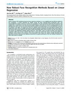
Figure 1: (a) is an input sample with contiguous occlusion. (b) is the sparse solution based on the OMP algorithm. (c) is the reconstructed image, whose class is the same as the class of the largest entry of the sparse solution. Obviously, the solution is not sparse enough and we have got a wrong answer due to the occluded part in 𝑦. 200 180 160 140 120 100 80 60 40 20 0
0
2000
(a)
4000
6000 All pixels
8000
10000
12000
(b)
Figure 2: Error between an occluded image and a “clean” one. We reshape the pixels in the two samples (a) into vectors and calculate the difference (b). Obviously, the distribution of error is like a comb, which indicates that the error exists in a few pixels and the others are “clean.”
4.1. Necessity of Preprocessing of Test Samples and Training Dictionary. When the test sample 𝑦 is occluded seriously, the error between 𝑦 and each column of 𝐴 increases, which means each element of vector 𝑒 rises, where 𝑒𝑖 = 𝑦 − 𝑎𝑖 . Hence, both the largest coefficient and the sparse level after some fix iteration times can hardly reach their respective predetermined thresholds. On condition that we employ 𝐴 and 𝑦 directly, as shown in Figure 1, the solution we get can be dense, which will surely weaken the superiority of sparse representation. Therefore it is necessary to process input sample 𝑦 and training dictionary 𝐴 firstly. It has been proposed that this kind of issue can be solved by block partitioning, which means to partition the image into blocks and process each block independently. The results for individual blocks are then aggregated. This method is only valid to images under contiguous occlusion. And the processing takes quite a long time since it transforms the classification to several subproblems. Let us think about how human brains handle the face images disguised by scarf or glasses. We make out the scarf or glasses in the image and then neglect these parts which are unrelated to face. And
our judgment of the person in the image depends on the other parts which we regard as face. Imitating the method human brain dealing with this kind of image, we can propose to preprocess the input image and training matrix before applying them to the OMP algorithm. No matter the random corruption or the contiguous occlusion part can be regarded as noise in the image, we can uniformly reject this part and only pay attention to the other parts.
4.2. How to Identify a Corrupted or Occluded Test Sample Automatically. Firstly, the system should automatically identify whether the test image is the one with partial occlusion or corruption. The errors between the occlusion and corruption image which belong to a class in the training dictionary or an invalid one are both quite large. But the error of an occluded one has some distinguishing features—the error between pixels focuses on only a few pixels; the others’ error is quite small. So if the error vector contained some elements which are closed to 0 and the variance of the error vector is
Mathematical Problems in Engineering
5
250 200 150 100 50 0 60
40 20 0 0
10
20
30
40
50
1 0.9 0.8 Coefficients
0.7 0.6 0.5 0.4 0.3 0.2 0.1 0
0
20
40
60
80
100
120
All images
Figure 3: Applying the occluded image (left top) directly to the algorithm, we get the wrong answer because part of the noise is too large for the system. By rejecting some pixels in the test image and shrinking the training matrix, respectively, the right person can be recognized.
large enough, 𝜎𝑒 > 𝜎0 , we can regard the test sample as a partial occlusion or corruption one, as shown in Figure 2. 4.3. Images Preprocessing to Corrupted or Occluded Samples. Then let us discuss how to use extract the “clean” pixels and remove the invalid ones. To begin with, we can define an error threshold 𝜉 between a particular pixel in test sample 𝑦 and respective pixels of elements in 𝐴. If the minimal error between the pixel in 𝑦 and respective pixel in one class of 𝐴 is larger than 𝜉, min (𝑦𝑖 − 𝑎𝑖𝑗 ) > 𝜉.
(13)
We can regard this pixel as an invalid one and remove it from 𝑦 as well as the respective one from 𝐴. Then we get the new training matrix 𝐴 1 and test vector 𝑦1 , whose “noise pixels” have been filtered. So the problem has been transformed into finding a sparse solution 𝑥1 subject to 𝑦1 = 𝐴 1 ⋅ 𝑥1 .
(14)
And the improved OMP algorithm can just be used in this new generated equation. One example is given in Figure 3. This will surely enhance the recognition rate of the system. Since this method does not involve any constraint conditions regarding noise distribution, the issue of random corruption and contiguous occlusion can be solved simultaneously. “Shrinking” of 𝐴 and 𝑦 also makes the computing speed faster.
5. Experimental Results In this section, we apply our algorithm on ORL database for face recognition. We first test the recognition rate and elapsed time of the algorithm, compared to the state-of-art algorithm to find the sparse solution. We then examine the identifying performance to corruption and occlusion. Finally, we simulate the real situation and check up the robustness under various disguises. 5.1. Performance on ORL Database and Yale Database. ORL database consists of 400 frontal images for 40 individuals. Samples in this database include facial variation like various expressions and postures, which can be obstacles or challenges for the system to find the true class of the test images. We test the face recognition rate and elapsed time of the algorithm by 10-fold cross-validation. In other words, for each test, the training dictionary is consisted of 40 classes of 360 images (9 samples per class) and the remaining 40 images are test samples. All these images have been simply downsampled, without any particular feature extraction. We compared the result with original OMP, together with some state-of-art algorithms aiming at sparse solution—primal augmented Lagrangian method (PALM), dual augmented lagrangian method (DALM), fast iterative soft-thresholding algorithm (FISTA), and truncated Newton interior-point Method (TNIPM). All results of each test and the average are in Table 1.
6
Mathematical Problems in Engineering Table 1: Comparison on ORL database.
Test number 1 2 3 4 5 6 7 8 9 10 Average(s)
PALM 1.0957 1.3422 1.5197 1.5638 1.2596 1.4026 1.3802 1.2477 1.4948 1.3220 1.3628
DALM 2.6292 2.6434 2.6408 2.6922 2.6749 2.6485 2.7209 2.7298 2.7602 2.6478 2.6788
Test number 1 2 3 4 5 6 7 8 9 10 Average
PALM 62.5% 70% 77.5% 80% 70% 77.5% 75% 67.5% 82.5% 75% 73.75%
DALM 87.5% 90% 92.5% 90% 92.5% 92.5% 92.5% 92.5% 95% 92.5% 91.75%
Elapsed time per test image(s) FISTA TNIPM 0.3548 0.9861 0.3628 1.0106 0.3607 0.9211 0.3661 0.9212 0.3655 0.8308 0.3635 0.8343 0.3682 0.8390 0.3742 1.0580 0.3635 0.8528 0.3670 1.04 0.3646 0.9294 Recognition rate FISTA TNIPM 90% 87.5% 90% 90% 92.5% 92.5% 92.5% 90% 92.5% 92.5% 92.5% 92.5% 95% 95% 92.5% 92.5% 95% 95% 95% 92.5% 92.75% 92%
OMP 33.1391 35.4203 34.7244 35.2557 36.5687 36.8514 36.7581 36.8528 35.9073 38.6038 36.008
Improved OMP 0.0278 0.0248 0.0233 0.0253 0.0238 0.0259 0.0218 0.0208 0.0213 0.0214 0.0236
OMP 77.5% 82.5% 80% 80% 85% 82.5% 87.5% 85% 85% 82.5% 82.75%
Improved OMP 95% 92.5% 95% 95% 97.5% 95% 95% 97.5% 97.5% 95% 95.5%
OMP 12.433 11.1681 11.3312 11.0440 10.5832 11.6463 13.0719 11.1364 11.5518
Improved OMP 0.7253 0.7690 0.7831 0.7920 0.7215 0.7824 0.6903 0.8467 0.6731
OMP 78.95% 81.58% 83.22% 85.53% 79.93% 82.89% 82.89% 86.51% 82.69%
Improved OMP 92.43% 92.76% 90.46% 95.72% 94.74 % 96.71% 92.43% 95.72% 93.87%
Table 2: Comparison on Yale database.
Test number 1 2 3 4 5 6 7 8 Average(s)
PALM 1.9440 1.6345 1.8704 1.9500 1.6420 1.3926 1.5375 1.3519 1.6654
DALM 1.3520 1.3967 6.3440 2.0409 1.3959 1.3948 1.3638 1.4371 2.0907
Test number 1 2 3 4 5 6 7 8 Average
PALM 52.96% 53.29% 51.97% 53.29% 47.37% 50% 49.34% 51.64% 51.23%
DALM 47.37% 50.33% 52.63% 51.64% 49.34% 51.64% 47.37% 50% 50.04%
Elapsed time per test image(s) FISTA TNIPM 5.9824 20.1194 6.4434 17.1639 6.3742 17.4002 7.0701 18.1936 6.1629 16.8426 6.1054 15.7372 7.3222 15.9961 7.8755 15.6780 6.6670 17.1414 Recognition rate FISTA TNIPM 92.11% 55.92% 95.39% 90.13% 92.76% 87.17% 92.43% 91.12% 94.41% 91.78% 96.38% 93.75% 93.42% 92.76% 95.39% 94.74% 94.04% 87.17%
Coefficients
Mathematical Problems in Engineering
1.2 1 0.8 0.6 0.4 0.2 0 −0.2
7
Recognition under varying level of corruption 100 0
20 40 60 80 100 120
90
Coefficients
1 0.9 0.8 0.7 0.6 0.5 0.4 0.3 0.2 0.1 0
1 0.9 0.8 0.7 0.6 0.5 0.4 0.3 0.2 0.1 0
80 Recognition rate (%)
Coefficients
All images
0
20 40 60 80 100 120 All images
70 60 50 40 30 20 10 0
0
10
20
30
40
50
60
70
80
90
Corrupted (%) Improved OMP OMP 0
20 40 60 80 100 120 All images
(a)
(b)
(c)
Figure 4: Recognition under random corruption. Left: (a) test images 𝑦 from ORL database, with random corruption. Top row: 30% of pixels are corrupted, middle row: 60% corrupted, bottom row: 90% corrupted. (b) Estimated sparse coefficients. (c) Reconstructed images. We can see that our algorithm outperforms the original OMP.
Table 3: Comparison on FERET database.
Test number 1 2 3 4 5 6 7 Average(s)
PALM 13.6277 13.6254 18.9904 15.2641 15.2024 13.1985 14.5053 14.9163
DALM 0.6245 0.6191 0.6191 0.6316 0.6364 0.6125 0.6365 0.6257
Test number 1 2 3 4 5 6 7 Average
PALM 40% 48.67% 45.33% 38.67% 44.67% 54.67% 42.67% 44.95%
DALM 90.67% 88% 65.33% 84.67% 86.67% 80% 90% 83.62%
Elapsed time per test image(s) FISTA TNIPM 3.7790 8.8048 3.8656 9.4325 3.8538 8.6242 4.0842 9.0337 4.0117 9.0880 3.8448 8.7168 3.7359 8.8999 3.8821 8.9428 Recognition rate FISTA TNIPM 92.67% 90.67% 92.67% 88% 68.67% 65.33% 88% 84.67% 92% 86.67% 86% 80% 93.33% 90% 87.62% 83.62%
OMP 10.1515 10.4445 10.2513 10.2262 10.4940 10.2518 10.8678 10.3839
Improved OMP 0.3854 0.3325 0.2858 0.3229 0.4109 0.4428 0.2599 0.3486
OMP 51.33% 50% 77.33% 72.67% 74.67% 57.33% 64% 63.90%
Improved OMP 93.33% 92% 92.67% 90.67% 93.33% 89.33% 94.67% 92.29%
Mathematical Problems in Engineering
Coefficients (a)
1 0.9 0.8 0.7 0.6 0.5 0.4 0.3 0.2 0.1 0
0.4 0.35 0.3 0.25 0.2 0.15 0.1 0.05 0 −0.05 −0.1
0.4 0.35 0.3 0.25 0.2 0.15 0.1 0.05 0 −0.05
Recognition under varying level of occlusion 100 0
20 40 60 80 100 120 All images
90 80 Recognition rate (%)
Coefficients
Coefficients
8
0
20 40 60 80 100 120 All images
70 60 50 40 30 20 10 0
0
10
20
30
40
50
60
70
80
90
Occluded (%) Improved OMP OMP 0
20 40 60 80 100 120 All images (b)
(c)
Figure 5: Recognition under varying levels of contiguous occlusion. (a) Top row: 30% occluded test sample, middle row: 60% occluded, and bottom row: 90% occluded. (b) Estimated sparse coefficients. (c) Reconstructed images.
As shown in Table 1, the recognition rate of improved OMP is the highest. Meanwhile, elapsed time per sample outperforms others. We also compared the algorithm with others in the Yale database. Yale database contains 2432 frontal images for 38 individuals, which were captured under various laboratorycontrolled lighting conditions. 8-fold cross-validation has been taken in this database, with 56 images of each class as training samples, and the other 304 images as test samples. Just as the tests on ORL database, the images have only been downsampled to construct the training dictionary to make the problem 𝐴𝑥 = 𝑦 become undetermined. The results of the 8 tests and average values are in Table 2. In Table 2, although the recognition rate of FISTA is higher than our algorithm, its run time is almost tenfold compared with the improved OMP. Similar experiments were performed on FERET database. Compared with the other face databases we mentioned above, this database includes more variations like postures and facial expressions. We ran 7-fold cross-validation, with 150 classes (6 samples per class) in this database as training database, the other 150 samples as test samples in each test. Data in Table 3 reflects the comparison of these algorithms. In Table 3, we can see that the average recognition rate of improved OMP is the highest in tests of FERET database and its run time is much shorter.
We get these data in MATLAB on a typical 2.40 GHz PC with quad-core processor. To be fair, both the training dictionary and the test samples are the same to all algorithms. And all identified results depend on the class of the largest coefficient in the sparse solution. The improved OMP algorithm greatly reduces the run time, and its recognition rates are relatively well. 5.2. Recognition despite Occlusion and Corruption 5.2.1. Recognition under Random Corruption. We first test the robust version of our algorithm for samples under random corruption. We add salt and pepper noise of different intensities to samples in the database to generate the test samples. Figure 4 plots the recognition results of the robust version of the OMP and applying OMP directly to the test samples. From Figure 4, when the face imaged is 90% corrupted by the noise, although we can hardly identify it as a face image, the algorithm still reconstructed the right image. The right line graph in Figure 4 indicates that this method performs quite well under the condition of large percent of random corruption. 5.2.2. Recognition under Continuous Occlusion. We add an irrelevant image with different sizes to the samples in the
Mathematical Problems in Engineering
9
Coefficients
(a)
0.45 0.4 0.35 0.3 0.25 0.2 0.15 0.1 0.05 0 −0.05
0
20 40 60 80 100 120 All images
0.9 0.8 0.7 0.6 0.5 0.4 0.3 0.2 0.1 0
0
20 40 60 80 100 120 All images
0.9 0.8 0.7 0.6 0.5 0.4 0.3 0.2 0.1 0 −0.1
0
20 40 60 80 100 120 All images
0.25 0.2 0.15 0.1 0.05 0 −0.05 −0.1
0
20 40 60 80 100 120 All images
(b)
(c)
Coefficients
(d)
0.7 0.6 0.5 0.4 0.3 0.2 0.1 0
0
20 40 60 80 100 120 All images
0.7 0.6 0.5 0.4 0.3 0.2 0.1 0
0
20 40 60 80 100 120 All images
0.7 0.6 0.5 0.4 0.3 0.2 0.1 0
0
20 40 60 80 100 120 All images
(e)
Figure 6: Continued.
0.4 0.35 0.3 0.25 0.2 0.15 0.1 0.05 0
0
20 40 60 80 100 120 All images
10
Mathematical Problems in Engineering
(f)
Figure 6: Recognition despite disguise like sunglasses, scarf, or respirator. (a) Test images with sunglasses or scarf. (b) Estimated sparse coefficients. (c) Reconstructed images. (d) Test images with sunglasses and scarf. (e) Estimated sparse coefficients. (f) Reconstructed images.
database and treat them as test image to test the robustness under continuous occlusion. Figure 5 indicates the performance. We can see in the right of Figure 5 that the improved OMP significantly outperforms the original one, which shows its robustness of occlusion. 5.3. Recognition despite Disguise. Face photos taken in a real world scenario often contained glasses and scarf, which makes it harder for the system to identify the right person. Now let us examine the performance of the algorithm under these kinds of situation. Our test images are also from ORL database and we add glasses and scarf pictures to the samples. Figure 6 shows that the algorithm also has a quite well performance on the real situation—disguised test samples. We constructed a disguised test sample database based on ORL database of 40 samples with sunglasses and scarf. And the recognition rate reached 95%.
6. Conclusions In this paper, we proposed a fast and robust algorithm based on OMP algorithm. We first discussed the disadvantage of OMP algorithm to solve the face recognition problem. Then an improved method is proposed to make the elapsed time become much shorter to identify a test image. We also tried to enhance robustness to the occluded and corrupted test samples by extracting the “noiseless” pixel and reduce the elements in both the test image and training dictionary, respectively. Finally, we prove this method by experiments on ORL database, Yale database, and FERET database. One further work is to enhance the robustness in situation under various kinds of misalignment and postures. We may further reduce the constrained condition and apply this method to object recognition.
Conflict of Interests The authors declare that there is no conflict of interests regarding the publication of this paper.
Acknowledgments This work was supported by National Natural Science Foundation of China (no. 61379010) and Natural Science Basic Research Plan in Shaanxi Province of China (no. 2012JQ1012).
References [1] J. Wright, A. Yang, A. Ganesh et al., “Robust face recognition via sparse representation,” IEEE Transactions on Pattern Analysis and Machine Intelligence, vol. 31, no. 2, pp. 210–227, 2009. [2] Y. Su, S. G. Shan, X. L. Chen et al., “Hierachical ensemble of global and local classifier for face recognition,” IEEE Transactions on Image Processing, vol. 9, no. 2, pp. 273–292, 2009. [3] A. Yang, A. Ganesh, S. Sastry, and Y. Ma, “Fast l1-minimization algorithms and an application in robust face recognition: a review,” in Proceedings of the International Conference on Image Processing, 2010. [4] J. Wright, Y. Ma, J. Mairal, G. Sapiro, T. Huang, and S. Yan, “Sparse representation for computer vision and pattern recognition,” Proceedings of the IEEE, vol. 98, no. 6, pp. 1031– 1044, 2010. [5] E. J. Cand`es, J. K. Romberg, and T. Tao, “Stable signal recovery from incomplete and inaccurate measurements,” Communications on Pure and Applied Mathematics, vol. 59, no. 8, pp. 1207– 1223, 2006. [6] E. J. Cand`es, J. K. Romberg, and T. Tao, “Stable signal recovery from incomplete and inaccurate measurements,” Communications on Pure and Applied Mathematics, vol. 59, no. 8, pp. 1207– 1223, 2006. [7] A. Martinez, “Recognizing imprecisely localized, partially occluded, and expression variant faces from a single sample per class,” IEEE Transactions on Pattern Analysis and Machine Intelligence, vol. 24, no. 6, pp. 748–763, 2002. [8] D. Donolo and M. Elad, “Optimal sparse representation in general(nonorthogonal) dictionaries via minimization,” Proceedings of the National Acadamy of Sciences of the United States of America, vol. 100, no. 5, pp. 2197–2202, 2003. [9] D. L. Donoho, “For most large underdetermined systems of linear equations the minimal 𝑙1 -norm solution is also the sparsest solution,” Communications on Pure and Applied Mathematics, vol. 59, no. 6, pp. 797–829, 2006.
Mathematical Problems in Engineering [10] A. M. Bruckstein, D. L. Donoho, and M. Elad, “From sparse solutions of systems of equations to sparse modeling of signals and images,” SIAM Review, vol. 51, no. 1, pp. 34–81, 2009. [11] S. S. Chen, D. L. Donoho, and M. A. Saunders, “Atomic decomposition by basis pursuit,” SIAM Review, vol. 43, no. 1, pp. 129–159, 2001. [12] A. Yang, M. Gastpar, R. Bajcsy, and S. Sastry, “Distributed sensor perception via sparse representation,” Proceedings of the IEEE, vol. 98, no. 6, pp. 1077–1088, 2010. [13] D. Donoho, A. Maleki, and A. Montanari, “Message-passing algorithms for compressed sensing,” Proceedings of the National Academy of Sciences, vol. 106, no. 45, pp. 18914–18919, 2009. [14] A. Beck and M. Teboulle, “A fast iterative shrinkagethresholding algorithm for linear inverse problems,” SIAM Journal on Imaging Sciences, vol. 2, no. 1, pp. 183–202, 2009. [15] F. Sanja, D. Skocaj, and A. Leonardis, “Combining reconstructive and discriminative subspace methods for robust classification and regression by subsampling,” IEEE Transactions on Pattern Analysis and Machine Intelligence, vol. 25, no. 3, 2006. [16] J. Wright and Y. Ma, “Dense error correction via ℓ1 -minimization,” IEEE Transactions on Information Theory, vol. 56, no. 7, pp. 3540–3560, 2010.
11
Advances in
Operations Research Hindawi Publishing Corporation http://www.hindawi.com
Volume 2014
Advances in
Decision Sciences Hindawi Publishing Corporation http://www.hindawi.com
Volume 2014
Journal of
Applied Mathematics
Algebra
Hindawi Publishing Corporation http://www.hindawi.com
Hindawi Publishing Corporation http://www.hindawi.com
Volume 2014
Journal of
Probability and Statistics Volume 2014
The Scientific World Journal Hindawi Publishing Corporation http://www.hindawi.com
Hindawi Publishing Corporation http://www.hindawi.com
Volume 2014
International Journal of
Differential Equations Hindawi Publishing Corporation http://www.hindawi.com
Volume 2014
Volume 2014
Submit your manuscripts at http://www.hindawi.com International Journal of
Advances in
Combinatorics Hindawi Publishing Corporation http://www.hindawi.com
Mathematical Physics Hindawi Publishing Corporation http://www.hindawi.com
Volume 2014
Journal of
Complex Analysis Hindawi Publishing Corporation http://www.hindawi.com
Volume 2014
International Journal of Mathematics and Mathematical Sciences
Mathematical Problems in Engineering
Journal of
Mathematics Hindawi Publishing Corporation http://www.hindawi.com
Volume 2014
Hindawi Publishing Corporation http://www.hindawi.com
Volume 2014
Volume 2014
Hindawi Publishing Corporation http://www.hindawi.com
Volume 2014
Discrete Mathematics
Journal of
Volume 2014
Hindawi Publishing Corporation http://www.hindawi.com
Discrete Dynamics in Nature and Society
Journal of
Function Spaces Hindawi Publishing Corporation http://www.hindawi.com
Abstract and Applied Analysis
Volume 2014
Hindawi Publishing Corporation http://www.hindawi.com
Volume 2014
Hindawi Publishing Corporation http://www.hindawi.com
Volume 2014
International Journal of
Journal of
Stochastic Analysis
Optimization
Hindawi Publishing Corporation http://www.hindawi.com
Hindawi Publishing Corporation http://www.hindawi.com
Volume 2014
Volume 2014