A Fast Technique for Vectorization of Engineering Drawings using Morphology and Digital Straightness Sekhar Mandal
Amit K. Das
Partha Bhowmick
Computer Science and Technology Bengal Engineering and Science University, Shibpur India
[email protected]
Computer Science and Technology Bengal Engineering and Science University, Shibpur India
[email protected]
Computer Science and Engineering Indian Institute of Technology, Kharagpur India
[email protected]
ABSTRACT A novel technique for vectorization of engineering drawings is presented. The novelty of the algorithm lies in exploiting certain digital-geometric properties of straightness to vectorize inclined line segments and curve segments after vectorizing the horizontal and the vertical pieces using the conventional morphological opening. The primitives, hence vectorized, are classified into (i) horizontal, (ii) vertical, (iii) inclined line segments, and (iv) curved segments. Such a classification expedites the reconstruction of an engineering drawing from the vector format. Experimental results on several benchmark datasets have been given to demonstrate its efficiency and elegance.
(a) A portion of an input document image containing text annotations embedded in the graphics.
Keywords Vectorization, Engineering drawings, Morphological opening, Digital straightness, Reconstruction.
1.
INTRODUCTION
Systems that can convert images of engineering drawing into vector format are in high demand today. A vectorized representation has multifaceted advantages like reduced memory requirement, ease of maintenance, and a hierarchical representation of their structure and content. Such a representation can readily be used for editing, browsing, indexing, and filing of document images [17, 18, 19]. Exclusive systems have been designed, therefore, over the last few decades, e.g., image and diagram extraction [6, 10], logo detection [2, 13], etc. Techniques for graphics recognition have also been proposed, which mostly perform line or curve recognition in one or two stages without any higher level processing [7, 14, 16]. An overview of these, along with their performance evaluation, may be seen in [18]. The focus of our work is vectorization of drawings after segmenting out the text from the document image. The first step of vectorization is to process the raster image in order to extract a set of lines, arcs, etc. Existing approaches
Permission to make digital or hard copies of all or part of this work for personal or classroom use is granted without fee provided that copies are not made or distributed for profit or commercial advantage and that copies bear this notice and the full citation on the first page. To copy otherwise, to republish, to post on servers or to redistribute to lists, requires prior specific permission and/or a fee. ICVGIP ’10, December 12-15, 2010, Chennai, India Copyright 2010 ACM 978-1-4503-0060-5/10/12 ...$10.00.
(b) Text annotations (shown in black) segmented out from the graphic part (shown in gray). Figure 1: Illustration of our procedure of textgraphics segmentation on a sample engineering drawing consisting of embedded text in a graphic component.
for detection of lines, arcs, etc. are mostly based on Hough Transform, which consumes a large amount of CPU time [5]. Other methods include skeleton-based approach [4], statistical and structural analysis [20, 21], predicate logic [9], etc. In our work, we have used tools from mathematical morphology to detect orthogonal (vertical and horizonal) line segments present in a graphic assemblage. Such morphological operators are endowed with high-speed output while extracting orthogonal segments with desired level of accuracy. After this, a novel digital-geometric technique is used to identify all the long-and-slanted line segments in the raster image as well as the arcs and arbitrary curve segments as sequences of short-and-continuous (piecewise) straight segments. Note that, our approach is different from “dominant point detection”; “dominant points” signify only high-curvature or terminal points, whereas our approach yields multiple vectors for a long curve although it may consist of only low-
(a) A portion of an input document image I containing text annotations embedded in the graphics.
(b) Text annotations (shown in gray) segmented out from the graphics part (shown in black) to obtain Ig .
(c) The image Ie containing the edge map obtained by Canny edge detection algorithm.
Figure 2: An illustration of the preprocessing in our algorithm on a sample engineering drawing present in a document image. curvature points (e.g., an arc of a digital circle with large radius). To reduce the error incurred by skeletonization, we have used Canny edge detection algorithm [1]. Thus, for each thick segment of a graphic piece, we have a pair of (orthogonal or inclined) straight or curved edges (as piecewise straight segments, owing to their discreteness), which, in turn, facilitates the reconstruction of an original graphics from its vector form. A brief outline of this paper is as follows. Section 2 describes the preprocessing, which results in the text-graphics segmentation followed by extraction of the graphics boundaries. After this, the proposed algorithm is presented in two parts: Section 3 is on morphological opening used to detect orthogonally straight pieces and Section 4 contains a brief discussion on digital straightness and how it is employed to vectorize straight and non-straight edges of arbitrary orientations and shapes. Section 5 points out the technicalities of reconstruction from the vector format, adopted in our algorithm. Section 6 shows some experimental results and the corresponding reconstruction errors. Finally, we conclude in Section 7 with the salient features of the algorithm and its future prospects.
2.
PREPROCESSING
The input to our algorithm is a gray-scale document image, denoted by I. By applying the texture-based technique given in [3], our algorithm first removes all half tones from the input image. Next, it is converted to a binary image Ib by the well-known technique proposed in [12], so that the text annotations embedded in the drawing are segmented out successfully from the binary image using the technique of [11]. Graphics segmentation using connected component analysis yields good results provided the lines and arcs constituting each graphical component are properly connected.
However, graphics consisting of dotted (or dashed or dotdashed) or short line segments are difficult to detect as the size of an individual component is similar to a text character. Hence, the individual connected component does not signify a meaningful graphics entity; whereas, a sequence (or group) of such components, taken together in an appropriate way, represents a substantive graphics component. Thus, the lesser part of the problem is detecting individual graphic elements, and the greater part lies in analyzing them for successful vectorization targeted to achieve the minimal output complexity. In order to perform the text-graphics segmentation from a binarized document image, Ib , we have used the procedure of [11]. A typical result of text segmentation from a graphics containing embedded text components is shown in Fig. 1. After removal of text annotations embedded in the drawing, the binary image is converted into a “pseudo gray-scale image”, namely Ig , by convolving the image Ib with a Gaussian filter of size 3 × 3. As mentioned earlier, the Canny edge detection algorithm is now applied on this pseudo gray-scale image for detection of edges of the graphic objects present in the image. Hence, we obtain the edge map Ie (a binary image) from Ig . A result after this preprocessing is shown in Fig. 2.
3.
STAGE I: MORPHOLOGY-BASED
The edge-mapped binary image Ie contains horizontal and vertical straight line segments apart from circular arcs and arbitrary curve segments, as mentioned earlier. In Stage I, we detect only the horizontal and the vertical line segments from Ie , using morphological opening, which works as follows: 1. Morphological opening operation with structuring element 1 × 4 is applied on Ie (The size 1 × 4 of the
(a) Horizontal line segments.
(b) Vertical line segments.
Figure 3: Horizontal and vertical line segments obtained by morphological open operation on the edge map shown in Fig. 2(c).
structuring element ensures that line segments having length less than 4 will not be recognized or vectorized.) 2. The length of each horizontal line segment is calculated; if the length of a segment is less than τhv (= 8 in our experiments), then the concerned line segment is discarded. The resultant image thus consists of horizontally straight segments each of length at least τhv , and is denoted by Ih . An output of this step is shown in Fig. 3(a).
Figure 4: Illustration of our procedure of detecting inclined straight pieces on a part of the engineering drawing in Stage II (Fig. 3).
It is evident that in the digital domain, each arbitrary arc may be considered to be piecewise straight, wherefore we may get some locally straight parts of an arc (which is actually not straight as a whole) as a horizontal line segment (Fig. 3(a)). This is really very difficult to predict using morphological tools, which is, however, taken care of in Stage II, where the notion of digital straightness can successfully determine long straight pieces of arbitrary orientation, thereby recognizing the rest as arbitrary curves. In order to detect vertical line segments, a similar procedure is repeated. Here the size of the structuring element is 4 × 1. The identified
eLip τw τw
vi
filled
vj
ej
p
ei
vj+1 vi+1
eR ip Case 1: There exists one horizontal edge ej within the vertical distance τw from ei and no edge on the other side of ei . Hence, ei and ej form two parallel edges (possibly partial) of a thick line segment.
eLip eLiq τw τw
vj vi
ej
p q ei vk ek
vj+1 vi+1 vk+1
R eR ip eiq
Case 2: There exist two edges within the vertical distance τw from ei ; the edge ej lies left and the edge ek lies right of ei . Hence, there arises an undecidability regarding the paired edge of ei . Figure 5: Vectorization of curved segments. Further results and the input image are shown in Fig. 7.
Figure 6: Cases considered in our algorithm of reconstruction.
vertical line segments are shown in Fig. 3(b) and stored in the image Iv . After identifying the horizonal and the vertical line segments, the image Ih ∪ Iv is subtracted from Ie to get the 0 0 resultant image Ihv = Ie r (Ih ∪ Iv ). The image Ihv consists of only inclined straight lines and arbitrary curve segments. We have identified the inclined line segments and as well as 0 the curved segments from the image Ihv , as explained next.
can be derived from the chord property. A curve C is digitally straight if and only if its chain codes have at most two values in {0, 1, 2, . . . , 7}, differing by ±1(mod 8), and for one of these, the run-length must be 1 (Property R1). Also, if s and n be the respective singular code and non-singular code in C, then the runs of n can have only two lengths, which are consecutive integers (Property R2). Properties R1 and R2 provide a sense of uniform direction related with straightness, since we have to “step along a digital line” mostly in a particular direction (out of eight possible) and occasionally in another (differing by 450 , since it’s the digital plane). However, the uniformity of the occasional change in direction is captured in Property R3, which is more stringent on digital straightness: One of the run lengths (i.e., of s) can occur only once at a time. Finally, the recursive way of defining uniformity of run-lengths of n is provided by Property R4: For the run length that occurs in runs, these runs can themselves have only two lengths, which are consecutive integers, and so on.
4.
STAGE II: DIGITAL-GEOMETRIC
0 A (digital) curve C ∈ Ihv is a sequence of pixels in 8Nconnectivity; i.e., (i, j) ∈ C and (i0 , j 0 ) ∈ C are neighbors of each other, provided max(|i − i0 |, |j − j 0 |) = 1, and the chain codes constituting C are from {0, 1, 2, . . . , 7} [8]. If each point in C has exactly two neighbors in C, then C is a closed curve; otherwise, C is an open curve having two pixels with one neighbor each, and the remaining pixels with two neighbors each. For a self-intersecting curve C, we split C into open or closed curve segments, as the case may be. In order to determine whether a segment C is straight or not, there have been several studies since 1960’s [8]. In [15], it has been shown that C is the digitization of a straight line segment if and only if it has the chord property.1 In this work, to detect a straight edge, some regularity properties of digital straightness have been used [15], which 1
C has the chord property if, for (p, q) ∈ C × C, p 6= q, for any (x, y) on the chord pq (real line segment joining p and q), ∃(i, j) ∈ C such that max {|i − x|, |j − y|} < 1.
4.1
Detecting Digitally Straight Pieces
0 It is evident that in the image Ihv obtained in Stage I, there may exist digital curve segments, which appear to be straight, but are not “exactly digitally straight” due the stricter digital-geometric properties of straightness, i.e., R3 and R4. Hence, in our algorithm, in order to detect approximately straight pieces, we have resorted to R1 and have done certain modifications for R2. We have dropped R3 and R4,
(a) Instance of an image Ie (after preprocessing).
(b) End-points (count = 178) of all the vectors.
(c) Reconstructed unfilled edges using the end-points.
Figure 7: Vector format and its edge-wise reconstruction for a text-segmented engineering drawing ‘e01’. See Fig. 8 for complete results. since they impose very tight restrictions to be accepted as digitally straight. Such a strategy has been made to successfully extract the (approximately) straight segments of arbitrary orientation, and some of its major advantages are as follows:
of n in C that determines the level of approximation, subject to the following two conditions:
• avoiding tight enforcing of digital straightness, especially for the curves which are possibly straight in the original drawing, but after digitization and subsequent processing, contains digital aberrations;
It may be noted that, in our approach of detecting approximately straight pieces of arbitrary orientations, we have strictly adhered to Property R1, since it is strongly related with the overall straightness of a digital curve segment. However, for R2, we consider that the run lengths of n can vary to an extent depending on the minimum run length of n. The reason for modifying R2 to the Condition C1 is that, in order to properly extract the approximately straight segments, we have permitted an allowance of approximation (d), which is realized by C1. Given a value of p, the amount d by which q is in excess of p indicates the deviation of the approximately straight piece from the actual/real line, since ideally (for an exactly straight piece) q can exceed from p by at most unity. Clearly, the error incurred is decided by d; lower the run length p of n, lower would be this allowance of approximation. So, we keep the provision for adaptively changing this allowance so that elongation of a detected straight piece is made as much as possible until it loses its overall approximate straightness. Another parameter incorporated in C2 is e, which, when coupled with C1, ensures that the extracted straight piece is not badly approximated due to some unexpected values of l and r. It may be noted that the properties R1–R4 do not give any idea about the possible values of l and r (depending on n) [8]. However, we have imposed some bounds on the possible values of l and r, in order to ensure a reasonable amount of straightness at either end of an extracted straight piece. The values of d and e considered in these conditions are chosen in a way so that they are computable with inte-
• reducing the number of output vectors; • reducing the run-time of detecting the straight pieces; • usage of integer operations only.2 0 Each digital curve segment C ∈ Ihv is characterized by the following sets of parameters:
1. orientations parameters given by n (non-singular element), s (singular element), l (length of leftmost run of n), and r (length of rightmost run of n), which play decisive roles on the orientation of the concerned curve, C. An example: For a curve segment having chain code 04 105 105 104 104 105 , we have n = 0, s = 1, l = 4, and r = 5. 2. run-length interval parameters given by p and q, where [p, q] is the range of possible lengths (excepting l and r) 2 No floating point operations are required; only integer operations for addition, shift, and comparison are necessary. Even multiplications and divisions have been avoided, e.g., to compute b(p + 3)/4c, 3 is added with p, followed by two successive right shifts.
(C1) q − p ≤ d = b(p + 1)/2c. (C2) (l − p), (r − p) ≤ e = b(p + 1)/2c.
(a) Input image of an engineering drawing after text segmentation.
(b) Output image after reconstruction from the vector format (Fig. 7c).
(c) Errors of reconstruction (red: positive error, blue: negative error).
Figure 8: Final output after reconstruction from the vector format (Fig. 7). ger operations only. Someone may also consider some other values, such as d = b(p + 3)/4c and e = b(p + 1)/2c, or so, provided it does not produce any undesirable result.
5.
RECONSTRUCTION
An engineering drawing is made up of straight and curved segments of varying thickness. We consider that the maximum thickness over all segments is τw , which serves as a search parameter in our algorithm. In our experiments, we have taken τw = 12. A thick segment S consists of two parallel sequences of edges — each edge being of one pixel 0 width — in Ih or Iv or Ihv . If, w.l.o.g., S is a horizontal segment, then its constituent horizontal edge pairs are all detected in Stage I. The set of all such horizontal edges is present in Ih , which is obtained from Ie (Sec. 3). We traverse the edges of Ih one by one, and find its nearest edge in Ih . Let ei (vi , vi+1 ) be the horizontal edge of Ih , which is currently under traversal. We compute the slope si of ei from its two end-points3 . While traversing ei from vi to vi+1 , we consider the orthogonal digital straight line of slope − s1i passing through each point p ∈ ei . We traverse from R p along each of the two directions, namely eL ip and eip , directed leftwards and rightwards w.r.t. ei (Fig. 6). In each direction, we traverse for a distance of at most τw , to search for a pixel of some other horizontal edge contained in Ih . While doing so, there may arise the following cases:
Case 1.
We reach a point from p0 along eL ip , which is one of the (end-) points, namely vj , of some other edge ej ∈ Ih . (In case p = vi , we may get some point other than an end-point of ej .) If no other edge is found to lie on the other side 3
si = 0 for each ei ∈ Ih , and 1/si = 0 for each ei ∈ Iv ; 0 however, we need si while considering ei ∈ Ihv .
of ei and within a vertical distance of τw from ei , then it implies that ej is the pairing edge of ei (Fig. 6). We compute the midpoint m of p and q and apply the flood filling algorithm in Ie with the right-neighbor point of m as the seed, to fill all the pixels lying inside the overlapped portion of the paired edges (shown in dark gray in Fig. 6). While filling, we mark all the edge points of ei and ej — which lie in the 4-neighborhood of a filled pixel — as ‘visited’, and do not consider these edge points for subsequent steps of reconstruction.
Case 2. There exist two (or more) edges within the vertical distance τw from ei ; the edge ej lies left and the edge ek lies right of ei (Fig. 6). This gives rise to an undecidability for pairing the edge of ei ; either ej or ek has to be be paired with ei but the decision is kept pending and possibly solved while ej or ek is traversed. Hence, we traverse the next edge ei+1 with no reconstruction based on ei .
Case 3. There is no edge in Ih parallel to ei ; so we traverse the next edge, ei+1 . 0 Similar treatments are done for edges of Iv and Ihv also, which finally produces the reconstructed output image J that closely matches the original image, I.
6.
EXPERIMENTAL RESULTS
We have implemented the algorithm in C on an Intel Core 2 Duo CPU E4500 2.20 GHz machine (Mandriva Linux 2008). We have tested the algorithm on several benchmark datasets containing gray-scale images of engineering drawings, one being http://www.iupr.org/arcseg2007. We have already shown some results in the previous sections. Fig-
(a) Input image (gray-scale, consists of 25351 object pixels after binarization in preprocessing: Sec. 2) of another engineering drawing.
(b) End-points (count = 659) of the vectors.
(c) Vectors reconstructed.
(d) Final image after reconstruction (error= 13.86%).
Figure 9: Results on another engineering drawing ‘g01’ (input source: http://www.iupr.org/arcseg2007). ure 7c shows how we get the edges for aiding the reconstruction from the vector format shown in Fig. 7b. In Fig. 8, we have given the result of final reconstruction using the intermediate edge map of Fig. 7b. To show the efficiency and accuracy of our algorithm, the error image is shown in Fig. 8c. The error of reconstruction in the reconstructed output image J is of the following types:
Positive error. A point p(i, j) corresponds to a positive error if and only if J[i][j] = 0 (i.e., background point) and I[i][j] = 1 (i.e., object point). Hence, total positive error in the output image J is given by |{(i, j) : I[i][j] = 1 ∧ J[i][j] = 0}|.
Negative error. p(i, j) corresponds to a negative error if and only if J[i][j] = 1 and I[i][j] = 0. Hence, total positive error in J is given by |{(i, j) : I[i][j] = 0 ∧ J[i][j] = 1}|.
In Fig. 8c, total error is 2856 points. The input image (Fig. 8a) consists of 19837 object points. Hence, the incurred error is 2856/19837 = 14.40%. Another set of experimental results is given in Fig. 9. It also shows how straight edges are successfully vectorized by our algorithm, irrespective of the lengths of the edges (notice the inclined edges). The curved segments, which are mostly circular arcs, require shorter vectors owing to the changing curvature, as evident from our experimental results. Table 1 presents a summary of results including CPU time for the images of Fig. 8, Fig. 9, and a few other images.
7.
CONCLUSION
We conclude this paper by reiterating the plus points of our approach. First and foremost, it is fully automatic with no manual intervention or parameter entry. The strength of morphological open operation in detecting horizontal and
Table 1: Experimental results for some images. image size N M % error CPU time (secs.) ×row +ve −ve SI SII total e01 394×610 19837 178 5.98 8.42 0.51 0.83 1.34 e02 480×624 21659 492 902 327 3.37 9.30 5.42 g01 988×784 25351 659 6.03 7.83 0.38 1.40 1.78 g02 740×634 1312 3.88 341 106 3.85 12.38 2.17 SI, SII: Stages I, II; N, M = # object points, # vector points.
[9]
[10]
[11] vertical line segments and the effectiveness of digital-geometric properties of straightness in obtaining the inclined straight edges as well as curved segments (as a sequence of piecewise straight segments) have been used in tandem to vectorize an engineering drawing after necessary preprocessing. As found by our experimental results, the reconstructed output is accurate up to 83%-88%. The level of accuracy obviously depends on several factors, such as amount of noise in the original gray-scale image, jaggedness of the curves and line segments, and the ratio of straight lines and curve segments. Further scope related with this work lies in designing a precision-based algorithm, which would take the maximal error of vectorization as input and hence report a vector format of lesser size as desired. Such a reduced vector format may be useful for fast cataloguing, browsing, and retrieval purposes of engineering drawings present in a large database of digital documents.
8.
[12] [13]
[14]
[15] [16]
[17]
REFERENCES
[1] B. Chanda and D. Dutta Majumder. Digital Image Processing and Applications. Prentice-Hall of India, New Delhi, 1999. [2] J. Chen, M. K. Leung, and Y. Gao. Noisy logo recognition using line segment Hausdorff distance. Pattern Recognition, 36(4):943–955, 2003. [3] A. K. Das and B. Chanda. Extraction of half-tones from document images: A morphological approach. In Proc. Int. Conf. on Advances in Computing, Calicut, India, Apr 6-8, pages 15–19, 1998. [4] P. Dosch, K. Tombre, C. Ah-soon, and G. Masini. A complete system for the analysis of architectural drawings. International Journal on Document Analysis and Recognition, 3:102–116, 2000. [5] P. Fr¨ anti, E. Ageenko, S. Kukkonen, and H. K¨ alvi¨ ainen. Using Hough transform for context-based image compression in hybrid raster/vector applications. J. Electron. Imaging, 11, 2002. [6] R. P. Futrelle, M. Shao, C. Cieslik, and A. E. Grimes. Extraction, layout analysis and classification of diagrams in PDF documents. In ICDAR ’03: Proc. Seventh Intl. Conf. Document Analysis and Recognition, pages 1007–1014, 2003. [7] G. J. Llados, E. Valveny and E. Marti. Symbol recognition: Current advances and prespectives. LNCS, 2390:104–127, 2002. [8] R. Klette and A. Rosenfeld. Digital Geometry: Geometric Methods for Digital Picture Analysis. Morgan Kaufmann Series in Computer Graphics and
[18]
[19]
[20]
[21]
Geometric Modeling. Morgan Kaufmann, San Francisco, 2004. R. G. L. P. Cordella, P. Foggia and M. Vento. Prototyping structure description: a inductive learning approach. In In Proceeding of the SSPR, pages 339–348, 1998. J. Li, A. Najmi, and R. M. Gray. Image classification by a two-dimensional hidden Markov model. IEEE Trans. Signal Process., 48(2):517–533, 2000. S. Mandal, S. P. Chowdhury, A. K. Das, and B. Chanda. An efficient method for graphics segmentation from document images. In Proc. ICAPR’07), pages 107–111, 2007. N. Otsu. A threshold selection method from gray-level histogram. IEEE Trans. SMC, 9(1):62–66, 1979. T. D. Pham. Unconstrained logo detection in document images. Pattern Recognition, 36(12):3023–3025, 2003. J.-Y. Ramel and N. Vincent. Strategy for line drawing understanding. In Proc. GREC 2003, LNCS, 3088:1–12, 2004. A. Rosenfeld. Digital straight line segments. IEEE Trans. Computers, 23(12):1264–1268, 1974. J. Song, F. Su, M. Tai, and S. Cai. An object-oriented progresssive-simplification-based vectorization system for engineering drawings: Model, algorithm, and performance. IEEE Trans. Pattern Analysis and Machine Intelligence, 24(8):1048–1060, 2002. S. Tabbone, L. Wendling, and K. Tomdre. Indexing of technical line drawing based on f-signature. In Proc. of ICDAR 2001, pages 1220–1224, 2001. Y. Wang, I. T. Phillips, and R. M. Haralick. Document zone content classification and its performance evaluation. Pattern Recognition, 39:57–73, 2006. L. Wenyin. On-line graphics recognition: State-of-the-art. In Proc. GREC ’03, volume 4958 of LNCS, pages 291–304, 2004. L. Wenyin, W. Zhang, and L. Yan. An interactive example-driven approach to graphics recognition in engineering drawings. International Journal on Document Analysis and Recognition, 9):13–29, 2007. A. K. C. Wong and M. You. Entropy and distance of random graphs with application to structural pattern recognition. IEEE Trans. PAMI, 7(5), pages 599–609, 1985.