PerfCenter: A Methodology and Tool for Performance Analysis of Application Hosting Centers Rukma P. Verlekar, Varsha Apte, Prakhar Goyal, Bhavish Aggarwal Dept. of Computer Science and Engineering Indian Institute of Technology Bombay Mumbai, Maharashtra, India Email:
[email protected],{varsha,prakhargoyal,bhavish}@cse.iitb.ac.in
Abstract— We present a tool, PerfCenter, that takes as input the deployment, configuration, message flow and workload details of the hardware and software servers in an application hosting center, and predicts the performance of the applications. We allow for a hierarchical specification of the data center, where software is deployed on machines, machines consist of hardware devices and are deployed on LANs. We also explicitly model network links between LANs and model the contention at those links due to messages exchanged between servers. While tools and methodologies for such analysis have been proposed earlier, our approach allows for the most natural specification of a “data center” architecture, and is best suited for aiding in design decisions regarding deployment and configuration of software on various hardware architecture scenarios. The tool takes this high level input and generates the underlying queueing network, which is then solved analytically. Since we allow for synchronous method calls, and model contention at software as well as hardware resources, the generated queueing network is solved using approximate methods. We validate the solution against results obtained from a measurement testbed, and found that the predicted values were reasonably accurate.
I. I NTRODUCTION The performance of online services has become one of the main quality attributes by which current Internet users rate them. A recent report by Jupiter Research [5], based on a study of on-line shoppers, identifies poor Web-site performance as second only to cost considerations, as a reason to entirely abandon, or not re-visit an online retailing Web-site. Thus, it is critical to offer good performance to Internet and Web users. Online services are typically supported by distributed applications, or “multi-tier” server systems. Thus, e.g., a Webbased e-mail service is supported by at least three application components, the Web server, IMAP server, and the SMTP server. More complex services can be made of a large number of such components. Such services are often hosted out of a “data center” which houses the machines running these applications. Before enabling such a service, the data center administrator has to make several decisions - how many hosts would be required for the service? How should the deployment of software components on hosts be? What should be the
configuration of an application (e.g. thread pool size). For larger organizations, a service could be composed out of applications that are geographically separated - in such a case, how would the network delay affect the user response time? All these questions can be answered by building an appropriate queueing model of the distributed system. However, given the complexity of multi-tier systems, such models cannot be built manually. Thus we need tools that can translate a highlevel specification of the distributed system into a queueing model, and then solve it. Over the last decade, there has been significant effort in creating tools and techniques for analysis of distributed systems [3]. All of the techniques are rooted in queueing theory, where the distributed system is viewed as a complex system of resources. The distributed system is mapped to a queueing network and analyzed. One of the primary challenges in such queueing network analysis has been the capturing of the “layered” behaviour of a distributed system - i.e. the behaviour in which the server of one queue, makes a request to another resource on behalf of the request that it is serving. This resource could be a hardware device (e.g. when a Web server thread joins a CPU queue), or another software server (e.g. when a Web server thread makes an RPC call to an application server). Several approaches have been proposed to solve such models. The significant ones include the Stochastic Rendezvous Network model by Woodside et al [14] and the Method of Layers by Sevcik and Rolia [12]. These approaches are notable for their analytical solutions of the models. The work in recent years has focussed immensely on translation of high-level specification, to the formalisms accepted by such models [10], [6], [7], [17], assuming that a tool for the solution of the model is available. Some amount of work has also been done in developing more accurate (as opposed to generic) models of a system, so that more detailed behaviour can be specified and analyzed [8], or in developing models specific to certain software technologies [11], [16]. While existing tools and techniques have progressed considerably, we believe there is still room for improvement in the ease with which some of the features of a distributed
system can be specified. Specifically, a direct approach by which a “data center architecture” can be specified would be very convenient. In other words, we would like to specify the hardware architecture (such as how many machines, of what type), the network architecture (how the machines are deployed on LANs, and perhaps separated by a WAN), the software architecture (the message flows for various use cases), and the deployment and configuration details of the software and hardware. To our knowledge, none of the existing tools/methodologies allow such specification. We introduce such a specification in the form of a software tool, called PerfCenter, which we believe is both intuitive and straightforward, and present the analytical methodology for derivation of various performance measures based on this specification. We validate the results of our tool with the actual measurements, and find that the model provides reasonable accuracy in predicting values of important performance measures of the distributed system. The rest of the paper is as follows: in Section II, we present a motivating example and review existing work in this area. We describe the elements of our system model in Section III. In Section IV, we present the formal specification and analytical solution of the model. In Section V, we present validation results, and illustrate the use of our tool by running various “what-if” scenarios. We conclude the paper in Section VI. II. M OTIVATING E XAMPLE : A W EBMAIL
SERVICE
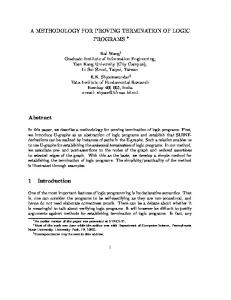
Consider a Web-based e-mail (Webmail) service, which is provided using the following software components: the Web, the Authentication, the IMAP and the SMTP servers. A typical Webmail service allows the user to login, on which it displays a list of messages from the user’s default folder. The user may then read, send, delete messages, and carry out a variety of other transactions on the IMAP/SMTP servers through the Web interface. Each arriving Web request triggers a flow of messages through the software components, which interact with each other to fulfill the user request. Each such type of request or a transaction is termed a use case scenario. A visual formalism called a Message Sequence Chart (MSC) [1] is often used to depict a use case scenario. Figures 1 and2 depict the MSCs corresponding to the login, read, send and delete scenarios for the Webmail system. In the login scenario, the Web server processes the user request and makes a call to the authentication server (send to auth) while passing on the user login id and password for authentication to it. The authentication server then verifies the credentials (verify password) and sends back the reply. We assume that the login request is rejected due to authentication failure with probability 0.1, whereas with probability 0.9 the user is authenticated. If authenticated, the Web server issues a request to the IMAP server to display the message box of the requesting user (send to imap). The IMAP server then sends the contents of the message box (list messages) to the Web server which formats it for sending it to the user (change to html). The rest of the scenarios are similar to the login scenario.
USER
W EB
AUT H
IMAP
USER
W EB
AUT H IMAP
sess id
password sta
sta vs
vp not ok cth
not ok cth
0.1
0.2 0.8
0.9
ok sti
ok sti
rm
lm cth
cth
(b)
(a)
Fig. 1. USER
W EB
Login and Read Message Scenarios
AUT H
IMAP SMT P USER
sess id
W EB
AUT H
sta
sta
vs not ok cth
vs not ok cth
0.1 0.9
ok sts
0.2 0.8
ok sti sm
cth
dm cth
(a)
Fig. 2.
IMAP
sess id
(b)
Send and Delete Message Scenarios
Several questions arise for this system, which depend on the hardware deployment and software configuration of the servers. E.g., for a given deployment, what would the bottleneck machine be? What would be the scenario response times? Would the machines be adequately utilized? How many threads should the Web-server be configured with? What if one of the servers is geographically separated? To answer such “what-if” questions, we would like a tool that would allow input specification in a manner that would be natural to a data center architect. In the following section, we review existing tools that try to meet this need. A. Existing Methodologies and Tools A large amount of research has been done over the last decade to address the problem of analyzing the performance of software systems. Here, we focus on approaches that propose analytical solutions to the performance models. The Method of Layers technique [12] was among the early approaches, which proposed a model and an analytical solution for capturing the “layered” behaviour of software systems - i.e. where one “layer” of servers uses the services of another layer of servers, where the lowest layer is that of
the hardware devices. All calls between layers are assumed to be synchronous. The Stochastic Rendezvous Network [14] is a powerful model, which captures many interesting behaviours of a distributed system. Apart from synchronous calls to servers at different layers, the model allows execution of a service in phases. This allows capturing of post-processing that is done by a server, even after a reply is sent back to the caller. The solution method of this model is implemented in a tool called the LQNSolver [15]. Further attempts have mainly focussed on mapping higher-level specification formalisms to the formalism that LQNSolver can accept (e.g. UCM2LQN [10], UML2LQN [17]). Some extensions to the “power” of the model have also been made (e.g. adding the capability of modeling forks and joins [10]) in the processing of the request. Another significant body of work has been done by Balsamo et al [1], [2], [4] who have used queueing networks with finite capacity queues to model software architectures, including those that allow synchronous calls between servers. After the initial efforts in defining stochastic models that could capture important behaviours, recent work has mainly been directed towards making specification easier for a software developer, so that the process of performance analysis can be integrated into the development cycle. A detailed survey is out of the scope of this paper, and the reader is instead referred to the excellent review by Balsamo et al [3]. While a variety of tools seem to exist for the purpose of analyzing software systems, we claim that none of these are suitable for analysis from the “data center” point of view. We claim that the existing tools are ideal as tools to be used during development, when the details of deployment may not be available. However, at the stage when an application is ready to be deployed in a hosting center, the architecture of the data center (machine specifications and network architecture) starts playing an important part. A data center architect would require a tool that allows him/her to run various what-if scenarios of deployment and configuration, and see their effect on the performance of the application. The formalism we propose captures the natural “language” that data center architects speak - in terms of number of machines of a certain type, the “specs” of a type of machine, the “deployment” of a software application on a certain machine, and the deployment of the machines on various different data centers that might be separated by long distance network links. PerfCenter accepts specification at this level, and solves the underlying queueing model which captures the complexity of the contention for resources. In the next section, we present the elements of our system model, which will clarify how our formalism is suited towards the analysis of an application that is about to be deployed in a data center. III. T HE D ISTRIBUTED S YSTEM M ODEL Our system model attempts to formalize a “data center” roughly hierarchically, as a typical architect would - thus we define machines, (software) servers, networks, and provide
1 resources CPU PS; 2 machines SUN[2]: CPU = 1; HP[2]: CPU = 1; 3 network lan1 lan2 trans=10MBps prop=2.3ms mtu=256B; 4 maplans lan1 SUN[1], SUN[2], HP[1], HP[2]; 5 software WEB: threads = 80 s t a {CPU = 0.015}, s t i { CPU = 0.020 }, s t s {CPU = 0.02}, c t h {CPU = 0.010}; AUTH: threads = 50 v p { CPU = 0.010 }, v s {CPU = 0.005}; IMAP: threads = 8 l m { CPU = 0.025 }, r m {CPU = 0.020}; SMTP: threads = 8 s m {CPU =0.014}; 6 mappings WEB SUN[1]; AUTH SUN[2]; IMAP HP[1]; SMTP HP[2]; Scenario Login 12.0 { WEB s t a AUTH v p 128 SYNC; [0.1] { AUTH v p WEB c t h 128 ; } [0.9] { AUTH v p WEB s t i 256 ; WEB s t i IMAP l m 512 SYNC ; IMAP l m WEB c t h 2048; } }
7
Fig. 3.
Example input file for the PerfCenter tool
finer level details of the resources that constitute the machines. We also specify deployment and configuration details for the servers. The deployment is specified in terms of servers on machines, and machines on LANs. The specification is done using a simple text interface. Figure 3 shows an excerpt from the input file corresponding to the example described in Section II. We explain the components of our system model using this input file as an example. 1) Hardware Devices: At the lowest level of the distributed system, there are hardware devices (e.g. CPU, disks), which are parts of machines. Each such device can be declared, by giving each type a symbolic name which is used later for referencing it and its corresponding service discipline (eg. PS for CPU, FCFS for Disk). 2) Machines: We can define different “types” of machines, and specify how many of each type there are in the system. A machine is defined by the types and the quantity of the various hardware devices (from the declared list) that it possesses. 3) Network Architecture: We allow our system to consist of several LANs that can be separated by point-to-point links. For each such point-to-point link we specify the value of transmission rate, propagation delay and the Maximum Transmission Unit (MTU). 4) Machine deployment description: The machines in the distributed system can be deployed onto different LANs. 5) Servers: Here, by “servers” we mean the server applications such as Web server, IMAP server, that run on the machines. Each of the servers in the distributed system is specified with the number of threads it possesses and its corresponding set of “simple” tasks. A “simple” task is defined as a continuous piece of execution, which holds a device of its host machine, for a given amount of time. (We will explain the concept of simple tasks further, in
Section IV). 6) Server deployment description: The deployment of these servers to different machines is also specified. 7) Use Case Scenarios: The interaction of the servers to provide a variety of services is specified through a formalism similar to message sequence charts which are a part of the UML specification. Each use case scenario consists of an ordered sequence of tasks of various servers, with certain annotations. Once a thread executes a task locally, it may make a synchronous or asynchronous call to a task of another server (denoted by a SYNC/ASYNC tag). We allow probabilistic branching to reflect different paths that may be taken in a scenario. We also have a notion of a message sent when a task makes a remote call. Thus each such call is annoted with a message size in bytes. The use case scenario itself is given a symbolic name and its corresponding arrival rate is specified in terms of requests per second. Thus, currently we assume “open” arrivals to the system. With the above specification, the performance measures of interest would be: • Response times of the use case scenarios • Utilization of the hardware resources • System capacity (in terms of maximum aggregate request rate that can be supported) • Bottleneck server (hardware or software). We derive all these measures using an analytical modeling approach that essentially views the entire system as a layered network of queues. The analytical methodology works by deriving two parameters: request arrival rate, and average service time, for each of the queues in the network. The arrival rate to each of the resources of the system depends on factors such as high-level use case scenario arrival rates, as well as the deployment of servers on machines, and machines on networks. The average service time of a server, in this case better termed as “holding time” of a resource is a complex quantity for this system: it depends on contention for resources that are requested while holding this resource - e.g. the holding time of a thread would depend on the time required for receiving a response from a remote server, when a synchronous call is made. It would also depend on the workload on the CPU on which the thread is executing - since there could be contention for the CPU. Thus, the methodology must take into account delays caused by all such interactions within the system. In the following section, we present in detail, the analytical solution for deriving the measures. Since it makes several assumptions along the way, the analytical solution is approximate.
that it is processing (e.g. in the Webmail example, the Web server calls the “list message” task of the IMAP server). This can be done in two ways. The first is to simply “forward” the request to the next server, without waiting for a response, thereby releasing the thread which was executing the request on this server. This is termed as an asynchronous call. The second way is to call the task of the other server, and wait for the response. In this case, the thread which makes the call, blocks, and is held until the response is received, and is continued to be held until either it makes an asynchronous call, or finishes processing and returns the response to the user (request exits). When we calculate queueing delays at software servers, the type of calls its tasks make is a very important factor that determines how long the thread resource is held by a request. • Simple vs Compound tasks: The tasks that a server carries out can be of two types: simple, and compound. Simple tasks consist purely of instructions that execute on local devices of the machine. Compound tasks represent functions or methods of servers that may not only have some local computation, but also include synchronous calls to other tasks. Thus, when a server thread performs a compound task, it is held during local computation as well as during the times that it is blocked on responses from synchronously called servers. E.g.,in the Webmail example, the Web server executes a compound call involving local processing (s t a, c t h, s t i) and synchronous calls to the authentication and IMAP servers. With the above clarification, we first proceed to formally express the specification given in the previous section, then derive the parameters of the underlying queueing network, and lastly, derive the performance measures of the queueing network. A. Formal model of the input parameters •
•
•
•
IV. T HE A NALYTICAL S OLUTION Before we present the formal model and solution of the queueing network underlying our system, we explain a few key concepts and definitions: • Synchronous vs asynchronous calls: A software server often calls a task of another server to fulfill the request
•
Let there be D types of devices, M machines and S servers in the system. A machine m is characterized by the set: {qm1 , qm2 , . . . , qmd , . . . , qmD } where qmd is the number of type d devices present in machine m. Two different machines that are characterized by the same set, are considered to be the same type of machine. Let A = [asm ] denote the server-to-machine allocation matrix. Thus, asm = 1 if server P s is deployed on machine m, and 0 if not. Then as = m asm denotes the number of machines on which server s has been deployed. Let B = [bmn ] denote the machine-to-LAN allocation matrix. Thus, bmn = 1 ifP machine m is deployed on LAN n, and 0 if not, with n bmn = 1. Further, let βm denote the index of the network on which machine m is deployed. Let rnn′ , δnn′ , and M T Unn′ denote the bit-rate, the propagation delay and the maximum packet size (“Maximum Transmission Unit”) respectively of the point-topoint link between the two LANs n and n′ .
Each server s is characterized by a simple task set: {E1s , E2s , E3s , . . . , Ens s }. We also specify the number of threads cs that the server can have. s • Associated with each simple task Et , is the execution time that it requires on each device d, denoted by τs,t,d • There are F use case scenarios in the system. The arrival rate of scenario f is denoted by λf . A use case scenario, f , is specified as a tree denoted as tf , where each node corresponds to a simple task and can be denoted by tfi . An arc from one node (task) to the next node (task) signifies that the first task has called the next task. Each such arc is annotated with the attributes: the probability of the call, whether the call is synchronous or asynchronous, and the size of the message transfered as a result of the call. Let G(tfi , tfj ) denote the probability that in scenario f , tree node tfi , representing task Ets , will call a tree node tfj , ′ representing task Ets′ . where tfi is an immediate parent node of tfj . N f is the total number of nodes in a tree for scenario f . The root of the tree is the first simple task of the scenario. • Let ls,t,s′ ,t′ denote the average size of the message sent ′ from task Ets to Ets′ in a scenario (thus, we assume that for a given sequence of one task calling another task, the average message size remains the same). The above structures and parameters form the input to our analytical model. •
•
j
i
ent node of tfj . If tfj is the root node then λtf =λf . Hence j the total arrival rate to any task Ets in a scenario f is PN f then j=1,tf =E s λftj . Since we assume that if the server t j is deployed on multiple machines, the load is equally distributed among all the servers, the total effective task PF PN f arrival rate will be λEts = f =1 j=1,tf =E s λftj /as . t j Assuming no probabilistic branching in scenarios, the arrival rate at a compound task, λTis is equal to the arrival rate of the first simple task in its execution sequence. s s s s s Thus, if Ti = Xi,1 , Xi,2 , Xi,3 , Xi,4 , . . . , Xi,Q s , where i s s s = λEts . This can be Xi,1 = Et then λTis = λXi,1 easily generalized to the case where there is probabilistic branching. The total arrival rate to a server s on a machine m is then given by X λsm = (1) λTis
B. Deriving the Parameters of the Queueing Network Based on the above input, some intermediate values need to be calculated, for deriving the performance measures of the system. Briefly, these values are the arrival rates and the average holding times that characterize the queueing models corresponding to the soft and hard resources of the system. Before deriving these quantitative parameters, the tool carries out the important step of identifying the compound tasks of a server. Recall that the tool user, in the specification, only provides details of the simple tasks of a server. The complete task set of a server is revealed only by inspecting the use case scenarios (algorithm given in [13]). Note that a simple task is a special case of a compound task, and thus, henceforth we refer to the compound tasks as simply “tasks”. Let the complete task set for the server s be denoted by T s = {T1s , T2s , . . . , TCs s }, where Cs is the total number of tasks in the task set of server s. Each task Tis in T s corresponds to an execution sequence of steps, which are either local computations (simple tasks) or synchronous calls. We s s s s s , . . . , Xi,Q , Xi,4 , Xi,3 , Xi,2 represent this as Tis = Xi,1 s where i s Qi is the total number of steps in the compound task Tis in Ts . s Xi,j is either a simple task Ets of server s or a synchronous ′ call to a task i′ of another server s′ , denoted by S(Tis′ ). We assume that every task consists of a simple task as its first step, possibly followed by an alternate sequence of synchronous calls and simple tasks. Once the task set for each server is built, we can proceed to derive the parameters of the various queueing models:
Task arrival rates: The task arrival rates to simple tasks, denoted by λEts are calculated based on the use case scenarios and their arrival rates. Using preorder tree traversal algorithm, we can calculate the total arrival rate to any simple task in a scenario by visiting each tree node. In a tree, node tfj represents task Ets and there can be many such nodes tfj1 ,tfj2 ,tfj3 ,. . .,tfjn . which also represent task Ets in the tree for any jn ≤ N f . Arrival rate to a particular node tfj which represents task Ets is λtf = λtf G(tfi , tfj ), where tfi is the immediate par-
i∈T s •
Thread holding times for each task: Let the holding time of task Tis , at machine m, be denoted by hsi,m . Then, Qsi X s s Rm (Xi,j ) (2) hi,m = j=1 s where Rm (Xi,j ) is either the response time at the devices s of a simple task or of a synchronous call. If Xi,j is a s simple task Et ,
s Rm (Xi,j )
=
D X
Rmd (Ets )
(3)
d=1
where Rmd (Ets ) is the response time of task Ets at device s is a synchronous call, say to task d on machine m. If Xi,j ′ s′ s Ti′ , then let Xi,j−1 be a simple task Ets , and let Ets′ be ′ the first simple task of Tis′ . Then the message size for this call is ls,t,s′ ,t′ , and the reply is of size ls′ ,t′ ,s,t . Then s ) is given by Rm (Xi,j P mesg mesg s′ m′ as′ m′ [Dm,m′ (ls,t,s′ ,t′ ) + Rm′ (Ti′ ) + Dm′ ,m (ls′ ,t′ ,s,t )] as′ if bmβm bmβm′ = 0, and by P s′ m′ as′ m′ Rm′ (Ti′ ) as′
(4)
(5)
•
•
The arrival rate of packets on the link (m, m′ ), λm,m′ is given by:
otherwise. ′ where Rm′ (Tis′ ) is the average response time of the (i′ )th mesg task of (s′ )th server on machine m′ , and Dm,m (ls,t,s′ .t′ ) mesg and Dm′ ,m (ls′ ,t′ ,s,t ) are the delays for transferring the message corresponding to the request and the response, respectively. Average thread holding time: The average thread holding time of server s at machine m, denoted by hsm is given by the weighted average of holding times of the individual tasks: PCs s s i=1 λTi hi,m s hm = P (6) Cs s i=1 λTi
XXXX s
λm,d =
asm 1(τs,t,d > 0)λEts
•
τm,d = •
PS
s=1
Pns
t=1
asm λEts τs,t,d
λm,d
(14) Thus, the link utilization ρm,m′ is given by λm,m′ lm,m′ /rm,m′ where lm,m′ /rm,m′ is the average packet transmission time. Given the average packet size, link rate and packet arrival rate, the link can be approximated as a simple M/M/1 queue, whose waiting time can be calculated. Let this waiting time be denoted by Wm′ m′ . The packet transfer delay of a packet of a particular size l is then simply given by Dm,m′ = Wm,m′ + l/rm,m′ + δm,m′ We approximate the message delay for a message of size L:
(7)
(8)
Arrival rates to links: Let λcall s,t,s′ ,t′ be the rate at which ′ a call is made to Ets′ from Ets . Then λcall s,t,s′ ,t′
=
f
f
X
N X
N X
f
i=1,tfi =Ets
′ j=1,tfj =Ets′
λtf G(tfi , tfj ) i
as
(9)
mesg Dm,m ′ (L)
= Wm,m′ + δm,m′ + L rm,m′ C. Performance measures The above analysis resulted in derivation of arrival rates and average holding times for all the queues in the model. Now, the performance measures of the system can be derived as follows: • Device throughput: Since we consider lossless queueing systems, device throughput, Λm,d is simply λm,d , if λm,d τm,d < qmd and qmd /τm,d otherwise. • Device utilization: The device utilization for a device d at machine m is given by λm,d τm,d (15) ρm,d = qm,d •
If denotes the total rate at which a server s sends messages to a server s′ , then XX t
λs,t,s′ ,t′
(10)
•
t′
The average number of packets generated between m and ′ m′ , by the call from Ets to Ets′ is nlink s,t,s′ ,t′ ,m,m′ = ceiling(
ls,t,s′ ,t′ ) M T Uβm,βm′
•
(11)
•
=
ls,t,s′ ,t′ nlink s,t,s′ ,t′ ,m,m′
(12)
(16)
where Wmd can be calculated by approximating the device as a simple M/M/c queue, with qmd servers, λm,d arrival rate, and τm,d service time. Server throughput: Again, since we consider lossless queueing systems, server throughput is simply Λsm = P λTis , if λsm hsm /cs < 1 and cs /hsm otherwise. Server utilizations: The utilization of a server s on machine m (denoted by ρsm ) is given by λsm hsm (17) cs Task response times: The task response times are given by Rm (Tis ) = hsi,m + Wm,s (18) ρsm =
The corresponding average packet size is given by pack ls,t,s ′ ,t′ ,m,m′
Device response times: These are given by: Rmd (Ets ) = Wm,d + τs,t,d
λcall s,s′
λcall s,s′ =
(13)
t′
λm,m′
s=1 t=1
where 1(τs,t,d > 0) is 1 if the Ets uses device d and 0 otherwise. Average device holding times: Although device holding times are given directly as an input, the average holding time of a device must be calculated, for characterizing the device-level queue. This average will depend on the relative arrival rates at which requests from various simple tasks with different holding times arrive to the devices. Hence the average holding time of a device d on machine m is given by
s′
and the overall average packet size, lm,m′ is given by: P P P P pack call link t′ asm as′ m′ ls,t,s′ ,t′ ,m,m′ λs,t,s′ ,t′ ns,t,s′ ,t′ ,m,m′ s t s′
Arrival rate to devices: The total arrival rate of simple tasks to a device of a machines is the sum of all the requests coming from all the tasks of all the servers deployed on that machine ns S X X
t
link asm as′ m′ λcall s,t,s′ ,t′ ns,t,s′ ,t′ ,m,m′
Ravg =
X λf Rf λf
500 Average scenario response time in ms
•
where Wm,s can also be calculated by approximating the software server as a simple M/M/c queue, with cs “servers”, λsm arrival rate, and hsm service time. Scenario response times: Without loss of generality, let us consider scenarios without probabilistic branching. The scenario can then be defined by a sequence of tasks. The scenario response time, Rf , then, is given by the sum of response times of all the tasks in the scenario. However, the response times of tasks that are called synchronously are not included in this sum, as they are already accounted for in the holding times of the calling tasks. The average scenario response time is the weighted sum of response times of all the scenarios, and is given by:
300
200
100
0
5
10
15
20
Arrival rate in requests per second
Fig. 4. Average scenario response time: comparison of model vs. measured values.
(19)
V. R ESULTS While there is a lot of work on models of distributed systems, very few report on their practical usability, which would depend greatly on the accuracy of the predictions of the model. We chose, therefore, to validate our model, with measured data. A testbed emulating the Webmail application as described in Section II was built, and experiments were carried out on it. The four different servers - Web, Authentication (Auth), IMAP and SMTP; were hosted on four different machines. The Web server is an Apache server executing PHP scripts to emulate synchronous calls to the Auth, IMAP and SMTP servers. The backend servers were written in C++. Multiple experiments were conducted on this distributed test-bed. For load generation, httperf [9] was used, while server performance measures were obtained through Linux utilities such as sar, ps, etc. The service times of the tasks in seconds were as specified in the input file of Figure 3. The mix of the request was as follows: one read and send request each is issued for every two logins. The measurements were carried out up to the point at which one of the servers bottlenecked. The values obtained for response time and CPU utilization were then matched against the results obtained from PerfCenter. Figures 4 and 5 compare the measured and model predicted values of average scenario response times and CPU utilizations, respectively, for the system specified in Figure 3, for varying load. The predicted CPU utilizations are highly accurate, while the the predicted scenario response times are also within reasonable accuracy up to the point where the Web server CPU reaches 80% utilization. This indicates that the model predictions are fairly reliable and can be used for making a number of deployment
400
0
100
f
Web-CPU Analytical Web CPU Mesurement Auth-CPU Analytical Auth CPU Mesurement Imap CPU Analytical Imap CPU Mesurement Smtp CPU Analytical Smtp CPU Mesurement
90 80 Utilization in percentage
Equations 2 to 18 can be solved iteratively till the corresponding values of thread holding times in the successive iterations converge, in order to yield the desired performance measures. The iteration starts with the initial values of waiting times set to zero. Thus, Wm,m′ , Wm,d and Wm,s should be set to 0.
Analytical Measurement
70 60 50 40 30 20 10 0 0
5
10
15
20
25
Arrival rate in requests per second
Fig. 5.
CPU utilization: comparison of model vs. measured values.
and configuration decisions by the data center architect. For example, it is clear from the utilizations that the machines hosting SMTP and Auth server are under-utilized, whereas the machine hosting the Web-server is over-utilized (100% at 22 requests/second). Thus, we could deploy the Web-server on two machines, while allocate only one machine to Auth and SMTP. Figure 6 shows the utilizations of the Web, AUTH and SMTP (both mapped to one machine) CPU’s under this scenario as predicted by PerfCenter. As we can see, the CPU utilizations are now balanced better, with the Web server CPU at 50% and the Auth and SMTP CPU at 23%, at 22 reqs/sec. Finally, we evaluate a scenario where the resource demands of simple tasks s t a and v s have been changed from 15ms to 55ms and 5ms to 55ms respectively. We still wish to support a maximum load of 22 req/sec. Here, we use PerfCenter to determine the optimal number of threads required to support this request rate. Too few threads may result in lesser capacity than required, and under-utilization of hardware resources, while too many threads are undesirable, since this implies system overheads. Thus, we evaluate the system with a varying thread configuration for the Web server. Figure 7 shows the change in Web CPU as well as the (software) server utilization with increasing number of threads for the server. We can see that as number of available threads increase, the CPU utilization and system throughput increases initially. After a certain point, however (after 19 threads), there is no benefit
55
acceptable by the tool. Furthermore, the tool needs to be validated on industrial-scale server appliations.
Web server CPU Auth, SMTP server CPU
50
Utilization in percentage
45
R EFERENCES
40 35 30 25 20 15 10 5 0 0
5
10
15
20
25
Arrival rate in requests per second
Utilization values with the new deployment.
100
25
80
20
60
15
40
10
20
5
0
System throughput
Utilization in percentage
Fig. 6.
0 0
1
2
3
4
5
6
7
8
9
10 11 12 13 14 15 16 17 18 19 20 21 22 23 24 25 26
Number of Web server threads Web server Web CPU
System throughput
Fig. 7. Using PerfCenter to find the minimum number of threads for the Web server for a system with higher resource demands.
in adding more threads - even though the server utilization decreases, the system throughput and CPU utilization flatten out. Thus the “optimal” number of threads for this workload is 19. VI. S UMMARY
AND
C ONCLUSIONS
In this paper, we introduced a system model that supports easy specification of data center design, and software architecture details, so that performance measures under various architecture, deployment and configuration options can be generated. We presented an analytical method for the approximate solution of the model. We compared our results with measured data, and found that the predicted results match quite well with the measured data. This tool can be a part of a more ambitious vision of selftuned systems, which optimize themselves for better performance. Several approaches have been proposed that utilize a modeling engine in a “control loop” for tuning system parameters. This tool could be used as one such engine. One of the drawbacks of this approach is that it requires detailed information about the system. This is an area of research we are actively focussing on - to auto-discover the message flows and resource consumption details that would serve as an input to this model. Once discovered, these inputs can be automatically converted into a specification format,
[1] F. Andolfi, F. Aquilani, S. Balsamo, and P. Inverardi. Deriving performance models of software architectures from message sequence charts. In WOSP ’00: Proceedings of the 2nd International Workshop on Software and Performance, pages 47–57, NY, USA, 2000. ACM Press. [2] Simonetta Balsamo, Federica Aquilani, and Paola Inverardi. An approach to performance evaluation of software architectures. In Proceedings of the first International Workshop on Software and Performance, pages 178–190, Santa Fe, New Mexico, United States, 1998. ACM Press. [3] Simonetta Balsamo, Antinisca Di Marco, Paola Inverardi, and Marta Simeoni. Model-based performance prediction in software development: A survey. IEEE Transactions on Software Engineering, 30(5):295–310, 2004. [4] Simonetta Balsamo and Moreno Marzolla. Performance evaluation of UML software architectures with multiclass queueing network models. In WOSP ’05: Proceedings of the 5th International Workshop on Software and Performance, pages 37–42, NY, USA, 2005. ACM Press. [5] Antone Gonsalves. Akamai and Jupiter Research identify ’4 seconds’ as the new threshold of acceptability for retail web page response times. TechWeb News, http://www.akamai.com/html/about/ press/releases/2006/press 110606.html, November 2006. [6] Vincenzo Grassi, Raffaela Mirandola, and Antonino Sabetta. From design to analysis models: a kernel language for performance and reliability analysis of component-based systems. In WOSP ’05: Proceedings of the 5th International Workshop on Software and Performance, pages 25–36, NY, USA, 2005. ACM Press. [7] Gordon P. Gu and D. Petriu. XSLT transformation from UML models to LQN performance models. In WOSP ’02:Proceedings of the 3rd International Workshop on Software and Performance. ACM Press, 2002. [8] Daniel A. Menasc´e; and Hassan Gomaa. A method for design and performance modeling of client/server systems. IEEE Transactions on Software Engineering, 26(11):1066–1085, 2000. [9] David Mosberger and Tai Jin. httperf: a tool for measuring web server performance. SIGMETRICS Performance Evaluation Review, 26(3):31– 37, 1998. [10] Dorin C. Petriu and C. Murray Woodside. Software performance models from system scenarios in use case maps. In TOOLS ’02: Proceedings of the 12th International Conference on Computer Performance Evaluation, Modelling Techniques and Tools, pages 141–158, London, UK, 2002. Springer-Verlag. [11] Paul Reeser and Rema Hariharan. Analytic model of web servers in distributed environments. In WOSP ’00: Proceedings of the 2nd International Workshop on Software and Performance, pages 158–167, NY, USA, 2000. ACM Press. [12] J. A. Rolia and K. C. Sevcik. The method of layers. IEEE Transactions on Software Engineering, 21(8):689–700, 1995. [13] Rukma P. Verlekar. Perfcenter: A methodology and tool for performance analysis of application hosting centers. Technical report, Department of Computer Science and Engineering, Indian Institute of Technology Bombay, 2007. [14] C. Murray Woodside, John E. Neilson, Dorina C. Petriu, and Shikharesh Majumdar. The stochastic rendezvous network model for performance of synchronous client-server-like distributed software. IEEE Transactions Computers, 44(1):20–34, 1995. [15] Murray Woodside. Layered queueing network solver. LQNSolver Homepage, http://www.sce.carleton.ca/rads/lqns/solver. html, November 1998. [16] Jing Xu, Alexandre Oufimtsev, Murray Woodside, and Liam Murphy. Performance modeling and prediction of enterprise javabeans with layered queuing network templates. In SAVCBS ’05: Proceedings of the 2005 Conference on Specification and Verification of Component-Based Systems. ACM Press, 2005. [17] Jing Xu, Murray Woodside, and Dorina Petriu. Performance Analysis of a Software Design Using the UML Profile for Schedulability, Performance and Time, volume 2794 of Lecture Notes in Computer Science. Springer, 2003.