A, FE

A STUDY OF THE WIND-DRIVEN OCEAN CIRCULATION IN AN EQUATORIAL BASIN by Mark A. Cane B.A.,

Harvard College, 1965

M.S., Harvard University, 1968

SUBMITTED IN PARTIAL FULFILLMENT OF THE REQUIREMENTS FOR THE DEGREE OF DOCTOR OF PHILOSOPHY at the MASSACHUSETTS INSTITUTE OF TECHNOLOGY August 1975 L~ L ~t~:

(A, -*~ FE r

Signature of Author-.

*'\

_

Department of Meteorology, August 1975

Certified by Thesis Supervisor Accepted by

Chairman, Departmental Committe

.NP

or Graduate Students

A STUDY OF THE WIND-DRIVEN OCEAN CIRCULATION IN AN EQUATORIAL BASIN by Mark A.

Cane

Submitted to the Department of Meteorology on 18 August, 1975 in partial fulfillment of the requirements for the degree of Doctor of Philosophy

ABSTRACT

A simple model has been developed to study the winddriven equatorial ocean circulation. It is a time dependent, primitive equation, beta plane model that is two-dimensional in the horizontal. The vertical structure consists of two layers above the thermocline with the same constant density. The ocean below the thermocline is taken to be of a higher constant density and to be approximately at rest. The surface layer is of constant depth and is acted upon directly by the wind. The depth of the lower active layer is dynamically determined. This is the simplest vertical structure which allows an undercurrent. The linear response of the model has been investigated thoroughly by analytic methods, as well as numerically. The nonlinear response has been studied numerically with the aid of some simple analytic arguments. The numerical scheme employs a variable mesh spacing, is fourth order in space and energy conserving (except for boundary effects). Small-scale noise is suppressed by a special treatment of the gravity wave terms. The linear responses to uniform southerly and easterly wind stress and the nonlinear responses to uniform wind stresses from the south, the east, the west, and the southeast have been studied numerically. The linear results are in agreement with analytic theory. In all cases, the surface flow is established within twenty days, a timescale determined by friction. There is also a timescale for the establishment of large-scale pressure gradients and mass transports. Linear theory shows that this "setup time" varies linearly with the time it takes for planetary waves to cross the ocean in the zonal direction. The nonlinear setup time can be either longer or shorter than the corresponding linear time, depending on the case, but in all cases would be six months or more for the world's oceans. Since this is at least as long as the timescale of the monsoonal wind systems, steady state theories should be applied to

equatorial oceans with caution. Flows become nonlinear within two weeks. A substantial amount of the energy put in at the surface by the wind stress is advected downwards by the strong vertical motions that arise near the equator. In the presence of meridional motions, exchanges of relative and planetary vorticity are dynamically significant. The nonlinear response to an easterly wind includes an eastward equatorial undercurrent in qualitative agreement with observations in many respects. In the linear response, the vertically integrated mass transport is westward at the equator. The flow that returns the undercurrent transport to the west takes place in the lower layer within 50 of the equator. The response to a west wind has eastward currents in both layers at the equator with a maximum at the surface. Both zonal wind cases exhibit variations in the zonal direction. It is argued that such variations are required by the dynamics in the absence of large frictional forces. The zonal mean state in response to a southerly wind has a narrow eastward jet at about 30 N and a broad area of westward flow at the equator. This state is barotropically unstable and after about 100 days westward propagating waves appear. With a southeast wind there is an eastward jet at 40 N and the mean position of the undercurrent shifts south of the equator. The undercurrent meanders with longitude but is steady in time. In this and the south wind case, the waves appear first at the western side of the basin and then spread eastward across the basin. There are no meanders in the zonal wind responses, suggesting that observed undercurrent meanders are instabilities of the equatorial current system as a whole and not of the undercurrent itself.

Thesis Supervisor: Title:

Jule G. Charney Sloan Professor of Meteorology

In memory of my mother

ACKNOWLEDGEMENTS I am grateful to my advisor, Professor Jule G. Charney, for his guidance and encouragement, and, most of all, for teaching me how to think about geophysical-phenomena. Several valuable conversations with Professor Henry Stommel are gratefully acknowledged.

My special thanks to

Dr. Edward Sarachik, who originally brought the subject area of this thesis to my attention and has provided invaluable criticisms throughout the course of this work.

It is a

pleasure to acknowledge Professor Eugenia Rivas for many hours of useful discussion about numerical methods.

I am

grateful to my fellow denizens of the fourteenth floor for their general camaraderie, as well as for a number of valuable conversations on various aspects of this work.

Dr.

Antonio Moura, Dr. Li-or Merkine and Mr. John Willett have been especially helpful. My thanks to Professor Dennis Moore for sharing his knowledge about equatorial waves.

I am grateful to Dr.

George Philander, Professor Walter Diing and Dr. Robert Knox for allowing me to see preliminary versions of their work.! The computations were carried out at the Goddard Institute for Space Studies and I am grateful to Dr. Robert Jastrow and Dr. Milton Halem for making this possible.

Many others at GISS provided needed assistance during the course of this work; special thanks to Ms. Ilene Shifrin, Mr. Leonard Keegan and Mr. Kenneth Woods.

My thanks, too,

to Ms. Sandy Congleton, Ms. Sylvia Wong and Ms. Helena Dinerman, who typed various drafts of this thesis. Some of the work reported in Chapter 4 was done in the summer of 1974, while I was a fellow in the Geophysical Fluid Dynamics program at the Woods Hole Oceanographic Institution, financially supported by NSF Grant GA-37116X. The larger part of my financial support was provided under NASA Grant NGR 22-009-727. I am happy to express my gratitude to my father for his unfailing faith and encouragement through the years. Most of all, I am grateful to my wife, Barbara, and my children, Laura and Jacob, for their patience and understanding, love and support, throughout the course of this work.

I owe them more than I can ever say. Finally, I would like to acknowledge my grandmother,

Rebecca Cohen, an inspiration, always.

TABLE OF CONTENTS

page Abstract

2

Dedication

4

Acknowledgements

5

Table of Contents

7

List of Tables

9

List of Illustrations

10

1.

Introduction

19

2.

Formulation of the Physical Model

27

2.1 2.2

27 37

3.

Linear Analytic Solutions

49

3.1 3.2

49

3.3 3.4 4.

5.

The Model Equations Choice of Parameter Values

Formulation of the Mathematical Problem Solution of the Steady State Interior Problem Sidewall Boundary Layers Solution of the Time Dependent Interior Problem

53 59 63

Time Dependent Forced Shallow Water Equations in an Equatorial Basin

69

4.1 4.2 4.3 4.4

69 71 76 94

Introduction Free Solutions Forced Response in an Unbounded Basin Forced Response in a Bounded Basin

Model Response to Simple Wind Stress Patterns

106

5.1 5.2 5.3

106 108

Introduction Linear Response to Nonlinear Response Wind 5.4 Linear Response to 5.5 .Nonlinear Response

a Uniform South Wind to a Uniform South a Uniform East Wind to a Uniform East Wind

138 180 214

page 5.6 5.7 6.

Nonlinear Respnse to a Uniform West Wind Nonlinear Response to a Uniform Southeast Wind

Summary and Conclusions

250 275 301

References

320

Appendix A

Eddy Viscosity

326

Appendix B

Numerical Methods

329

B.1 B.2 B.3 B.4 B. 5 B. 6

Variable Grid Time Differencing Spatial Differencing: Approximations Spatial Differencing: Gravity Wave Terms Summary

Appendix C Plane

329 330 Finite Difference Conservation Form

332 335 344 351

Finite Difference Equations on a Beta 353

Appendix D Computational Stability (Linear Analysis)

359

Appendix E

363

E.1 E.2

E.3

Computational Formulas for Chapter 4

Properties of the Hermite Functions The Projections of the Forcing Functions Boundary Response Terms

363 364 365

Appendix F Orthogonality and Completeness of the Eigenfunctions for the Shallow Water Equations

369

Biographical Note

372

LIST OF TABLES page Table 1

Non-dimensionalization of Variables

Table 2

Position of Points in the Standard Grid

48

LIST OF ILLUSTRATIONS1 Figure

Page

2.1

Multi-layer model.

28

2.2:

Model with Lwo active layers.

28

4.1

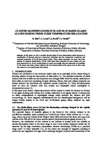
Dispersion relation for waves on an equatorial beta plane.

74

Response to F=l, G=Q=0 in an unbounded basin; see Equation (4.19).

83

Response to F=0, G=i, Q=0 in an unbounded basin.

85

4.2 4.3

5.1 5.2

Schematic view of linear adjustment to a south wind. Energies from 150S to 15 0 N.

Linear.

South wind. 5.3 5.4a 5.4b 5.5 5.6a 5.6b 5.6c

117

Energies from 5.60 S to 5.6 0N. South wind. us vectors at 8 days. South wind. u

1

vectors at 8 days. South wind.

u vectors at South wind.

G16 days.

u s vectors at 40 days. ~ South wind. u

1

Linear. 118

Linear. 120 Linear. 121 Linear. 124

Linear. 126

vectors at 40 days. South wind.

Linear.

h contours at 40 days. South wind.

Linear.

1

114

127

128

Some explantory material related to the computerproduced figures may be found in Section 5.1.

page 5.7a 5.7b 5.7c 5.8 5.9a 5.9b 5.9c 5.10 5.11 5.12 5.13 5.14 5.15 5.16a 5.16b 5.17

Meridional sections of h to day 398 at x=25.4 0 . Linear. South wind.

129

Meridional sections of h to day 398 at x=14.3 0 . Linear. South wind.

130

Meridional sections of h to day 398 at x=3.2 0 . Linear. South wind.

131

Meridional sections of u to day 398 at x=14.3 0 . Linear. South wind.

132

u s vectors at 398 days. South wind.

134

u

1

Linear.

vectors at 398 days. South wind.

Linear.

h contours at 398 days. South wind.

Linear.

u vectors at 398 days. South wind.

135 136 Linear. 137

Energies from 150 S to 150 N. South wind. Energies from 5.60S to 5.60 N. linear. South wind. u

Nonlinear. 140 Non-

contours at the equator to day 398. Nonlinear. South wind.

h contours at 8 days. South wind.

Nonlinear.

u contours at 8 days. South wind.

Nonlinear.

143 145 146

u s vectors at 16 days. South wind.

Nonlinear.

ul vectors at 16 days. ~ South wind.

Nonlinear.

u vectors at 16 days. South wind.

141

148 149 Nonlinear. 150

page 5.18a 5.18b 5.18c 5.19 5.20a 5.20b 5.20c 5.21a 5.21b 5.21c 5.22a 5.22b 5.23a 5.23b 5.23c 5.24

u s vectors at 40 days. South wind.

Nonlinear.

u' vectors at 40 days. South wind.

Nonlinear.

h contours at 40 days. South wind.

Nonlinear.

151 152 153

h contours at 119 days. South wind.

Nonlinear.

us vectors at 159 days. South wind.

Nonlinear.

u

vectors at 159 days. South wind.

Nonlinear.

h contours at 159 days. South wind.

Nonlinear.

us vectors at 398 days. South wind.

Nonlinear.

u

1

164 165 166 167 169

vectors at 398 days. South wind.

Nonlinear.

h contours at 398 days. South wind.

Nonlinear.

u contours at 398 days. South wind.

Nonlinear.

v contours at 398 days. South wind.

Nonlinear.

170 171 172 173

Meridional sections of h to day 398 at x=25.4 0 . Nonlinear. South wind.

176

Meridional sections of h to day 398 at x=14.30 . Nonlinear. South wind.

177

Meridional sections of h to day 398 at x=3.2 0 . Nonlinear. South wind.

178

Meridional sections of u to day 398 at x=14.3 0 . Nonlinear. South wind.

179

page 5.25 5.26 5.27 5.28 5.29 5.30 5.31a 5.31b 5.31c 5.32a

Energies from 15*S to 150 N. Linear. East wind.

186

Energies from 5.60S to 5.60 N. Linear. East wind.

187

Sections of h along the equator to day 38. Linear. East wind.

189

Sections of h along the equator to day 398. Linear. East wind.

190

Sections of u along the equator to day 38. Linear. East wind.

191

Sections of u along the equator to day 398. Linear. East wind.

192

Meridional sections of h to day 397 at x=25.4 0 . Linear. East wind.

195

Meridional sections of h to day 397 at x=14.3 0 . Linear. East wind.

196

Meridional sections of h to day 397 at x=3.2 0 . Linear. East wind.

197

u s vectors at 16 days. East wind.

199

Linear.

1

5.32b 5.32c 5.33a 5.33b 5.33c 5.33d

u

vectors at 16 days. East wind.

Linear.

h contours at 16 days. East wind.

Linear.

u s vectors at '40 days. East wind.

Linear.

ul vectors at 40 days. ~ East wind.

Linear.

h contours at 40 days. East wind.

Linear.

u vectors at 40 days. East wind.

200 201 202 203 204 Linear. 205

14 page 5.34a 5.34b 5.35a 5.35b 5.35c 5.35d 5.36 5.37 5.38 5.39 5.40 5.41 5.42a 5.42b 5.42c 5.43

h contours at 200 days. East wind. u vectors at 200 days. East wind. us vectors at 397 days. East wind. u

1

Linear. 206 Linear. 207 Linear. 208

vectors at 397 days. East wind.

Linear.

h contours at 397 days. East wind.

Linear.

u vectors at 397 days. East wind.

209 210 Linear. 211

Energies from 150 S to 150 N. Nonlinear. East wind.

216

Energies from 5.60S to 5.60 N. Nonlinear. East wind.

217

Sections of h along the equator to day 40. Nonlinear. East wind.

219

Sections of h along the equator to day 398. Nonlinear. East wind.

220

Sections of u along the equator to day 40. Nonlinear. East wind.

222

Sections of u along the equator to day 398. Nonlinear. East wind.

223

Meridional sections of h to day 398 at x=25.41. Nonlinear. East wind.

225

Meridional sections of h to day 398 at x=14.30 . Nonlinear. East wind.

226

Meridional sections of h to day 398 at x=3.2 0 . Nonlinear. East wind.

227

Meridional sections of u to day 40 at x=14.3 0 . Nonlinear. East wind.

229

15

page 5.44 5.45a 5.45b 5.45c 5.46a 5.46b 5.46c 5.46d 5.47a 5.47b 5.47c 5.47d 5.48 5.49 5.50 5.51

Meridional sections of u to day 398 at x=14.3 0 Nonlinear. East wind.

230

us vectors at 16 days. East wind.

Nonlinear. 231

u

vectors at 16 days. East wind.

Nonlinear.

h contours at 16 days. East wind.

Nonlinear.

us vectors at 40 days. East wind.

Nonlinear.

ul vectors at 40 days. East wind.

Nonlinear.

h contours at 40 days. East wind.

Nonlinear.

u vectors at 40 days. ~ East wind.

232

235 236 237 Nonlinear. 238

u s vectors at 400 days. East wind.

Nonlinear.

u

vectors at 400 days. East wind.

Nonlinear.

h contours at 400 days. East wind.

Nonlinear.

u vectors at 400 days. East wind.

233

239 240

Nonlinear.

241 242

Energies from 15 0 S to 1 50N. Nonlinear. West wind.

252

Energies from 5.60 S to 5.60 N. Nonlinear. West wind.

253

Sections of h along the equator to day 40. Nonlinear. West wind.

255

Sections of h along the equator to day 398. Nonlinear. West wind.

256

page 5.52 5.53 5.54a 5.54b 5.54c 5.55 5.56 5.57a 5.57b 5.57c 5.58 5.59a 5.59b 5.59c 5.59d 5.60

Sections of u along the equator to day 40. Nonlinear. West wind.

257

Sections of u along the equator to day 398. Nonlinear. West wind.

258

Meridional sections of h to day 398 at x=25.4 0 . Nonlinear. West wind.

260

Meridional sections of h to day 398 at x=14.3 0 . Nonlinear. West wind.

261

Meridional sections of h to day 398 at x=3.2 0 . Nonlinear. West wind.

262

Meridional sections of u to day 40 at x=14.3 0 . Nonlinear. West wind.

263

Meridional sections of u to day 398 at x=14.3 0 . Nonlinear. West wind.

264

u s vectors at 16 days. West wind.

266

1

Nonlinear.

vectors at 16 days. West wind.

Nonlinear.

h contours at 16 days. West wind.

Nonlinear.

u

u vectors at 40 days. West wind.

267 268 Nonlinear. 270

u s vectors at 398 days. West wind.

Nonlinear.

vectors at 398 days. West wind.

Nonlinear.

h contours at 398 days. West wind.

Nonlinear.

u

u vectors at 398 days. West wind.

271 272 273 Nonlinear.

Energies from 150 S to 150 N. Nonlinear. Southeast wind.

274 277

page 5.61 5.62 5.63a 5.63b 5.63c 5.64a 5.64b 5.64c 5.65a 5.65b 5.65c 5.66a 5.66b 5.67

5.68a

Energies from 5.60 S to 5.60 N. Nonlinear. Southeast wind. u

1

contours at the equator to day 398. Nonlinear. Southeast wind.

u s vectors at 16 days. Southeast wind.

Nonlinear.

u I vectors at 16 days. Southeast wind.

Nonlinear.

u vectors at 16 days. Southeast wind.

282 Nonlinear. 283 Nonlinear.

u

vectors at 40 days. Southeast wind.

Nonlinear.

h contours at 40 days. Southeast wind.

Nonlinear.

284 285 286

vectors at 398 days. Southeast wind.

Nonlinear.

vectors at 398 days. Southeast wind.

Nonlinear.

h contours at 398 days. Southeast wind.

Nonlinear.

u contours at 398 days. Southeast wind.

Nonlinear.

v contours at 398 days. Southeast wind.

Nonlinear.

u

I

279 281

u s vectors at 40 days. Southeast wind.

u

278

288 289 290 291 292

Meridional sections of u to day 398 at x=14.3 0 . Nonlinear. Southeast wind.

295

Meridional sections of h to day 398 at x=25.40 . Nonlinear. Southeast wind.

296

18

page 5.68b

Meridional sections of h to day 398 at x=14.3 0 . wind.

5.68c

Nonlinear.

Southeast 297

Meridional sections of h to day 398 at x=3.2 0 . Nonlinear. Southeast

wind.

298

1.

Introduction Since the vertical component of the Coriolis force van-

ishes at the equator, the geostrophic balances which dominate the dynamics of the extra-equatorial oceans must break down. The most striking physical manifestation of this singularly is the Equatorial Undercurrent, a narrow (half width of 10),

fast

(speeds up to 170 cm/ sec), eastward flowing subsurface current in the thermocline of all the world's oceans.

(While it is a

permanent feature in the Atlantic and Pacific at most longitudes, it has been observed only intermittently in the Indian Ocean.)

Many of the characteristics of the undercurrent are

highly variable:

e.g., the downstream velocities and trans-

ports may vary by a factor of two or more at different longitudes or at different times.

Available observational data

allows many of these variations to be related systematically to variations in the winds over the equatorial ocean.' However, the evidence is, in general, too spotty to allow such correlations to be conclusive.

Philander (1973b) presents a thorough

review of the measurements of the undercurrent made up to 1973. An important series of measurements of the undercurrents in the Atlantic was

made during the GATE exeriment in the summer of

1974.

(Preliminary results are available in Duing et.al.,

1975).

The most important finding was a meandering of the

undercurrent core between 11S and 1ON at all observed longitudes between July 26 and August 19.

The period of these

meanders was about 18 days. A second important consequence of the vanishing of the

Coriolis term is that equatorial motions have time scales which are very much shorter than those of midlatitude motions: the baroclinic time scale is weeks at the equator, as against years at mid-latitudes.

The most impressive instance of this

short time scale is the reversal in direction of the Somali Current within a month of the onset of the southwest Monsoon (e.g., Leetmaa 1973).

In general, time dependent.oceanic

motions with zime scales longer than a few days have received relatively little attention.

Equatorial regions are rewarding

areas for the study of such time variations because of the rapidity of the ocean's response to atmospheric forcings.

The

Indian Ocean is particularly favorable because, while the wind systems over the Atlantic and Pacific Oceans have monsoonal components, the monsoon regime is Ocean.

predominant over the Indian

The winds there reverse direction completely twice a

year and the currents are known to vary greatly.

NeVe-.theless

there have been few theoretical studies of time depEr phenomena in equatorial oceans.

t

Cox (1970) and Lighthll1

(1969) investigated the setup of the Somali Current in rcrDonse to the onset of the Southwest Monsoon.

On the basis of a

numerical simulation, Cox concluded that the Somali Current began to flow northward in response to the local winds along the African coast.

Lighthill's analytic model suggested that

the propagation of signals from the interior of the ocean could be the causal mechanism.

Gill (1972) applied a Light-

hill-like model to the undercurrent in the western Pacific. He associated the undercurrent with the second baroclinic mode

21 Kelvin wave which propagates in from the western boundary.

It

is not clear how such a model explains the presence of the undercurrent as a more permanent feature. In contrast to the situation for time varying equatorial currents, numerous theoretical models for the steady state undercurrent appear in the literature.. These have recently been reviewed by both Gill (1972) and Philander (1973b).

For

this reason we shall forego a detailed review here; rather, we shall discuss them only to the extent needed to establish a theoretical context for the present work. observations in the Pacific, Knauss

On the basis -of his

(1966) estimated that the

only negligible terms in the momentum equation were those giving the time rate of change of momentum and the horizontal component of the Coriolis force due to vertical motion. did not consider horizontal eddy diffusion processes.)

(He The

upshot is that a great variety of processes are available to be used as explanations for the undercurrent.

Since there is a

certain amount of freedom in the choice of eddy coefficients, all of these can be expected to give agreement with at least some of the observed scales.

In what follows, we seek to iso-

late those processes which are most significant. We shall immediately restrict ourselves to those models which idealize the thermocline as a discontinuity between a shallow upper homogeneous layer and a deeper lower homogeneous layer of greater density.

The lower layer is assumed to be so

deep that its horizontal pressure forces and velocities vanish. As shown by Charney (1955) the upper layer of such a model is

22 equivalent to a single layer homogeneous ocean with the force of gravity reduced by a factor Ap/p, the relative density difference between the two layers.

Models with thermohaline

components ,(Robinson 1960, Philander 1972, 1973a) are required to explain certain effects at depth; for example, the double celled structure often observed in the Pacific (see Philander 1973b).:

Homogeneous models appear to be sufficient for ex-

pla-in-ing observed features above the thermocline. The-most basic physical notion about the undercurrent is the idea of flow down a pressure gradient (Charney 1960). The prevailing easterly winds pile up water at the western side of the -ocean basin, thus establishing an eastward pressure gradient.

.Stommel (1960) exploited this idea to obtain an

eastward flowing subsurface current in a linear model with vertical friction.

He assumed free slip boundary condition at

the bottom .and that the vertically integrated transport van-ishes at the equator.

In a similar model without the latter

two assumptions, Charney (1960) and Philander (1971) found that the current at the equator did not reverse with depth.

In any

case, one would wish any theory to account for the substantial eastward transports observed at the equator.

in the linear

theory of Gill (1971), the pressure gradient force is balanced by the horizontal mixing of momentum.

By using an unrealisti-

cally large value for the coefficient of horizontal eddy viscosity (108 cm2 sec-1), Gill obtains the observed latitudinal scale for the undercurrent, but the transport is too low by a factor of at least four.

Non-linear theories have ignored the downstream inertial terms,.

The (suspect) assumption is made that the zonal and

meridional velocities have the same scale.

Then, since the

meridional length scale (an equatorial boundary layer scale) is so much shorter than the zonal one (the length of the basin),

it follows that in the momentum equation the downstream

inertial term is negligible relative to the cross-stream inertial term. circulation.

Attention is then directed to the meridional

For an -easterly wind, the Ekman drift in the

surface layers will be poleward.

Continuity then requires-a

compensatory equatorward mass flux at depth, producing an upwelling region at the equator to complete the fluid circuit. Fofonoff and Montgomery (1955) considered the subsurface flow in the light of the barotropic vorticity equation.

If it is

assumed that a parcel approximately conserves the vertical component of its absolute vorticity, it must change- its relative vorticity to make up for the loss of planetary vorticity as it moves equatorward. the equator.

This results in an eastward flow at

It may also be shown that the meridional circu-

lation near the equator enhances the eastward transport at the equator regardless of whether the wind is easterly or westerly. (See Robinson (1966) for an analytic demonstration; Gill (1972) gives a more physical argument.) The models of Charney (1960), Charney and Spiegel (1971), Robinson (1966), and McKee (1973) all incorporate the nonlinear effects due to the circulation in the meridional plane.

The first three

include momentum mixing in only the

24 ,vertical direction.

McKee's model is an extension.of Gills

(1971) -model into the non-linear regime; horizontal -eddy viscosity is the important frictional force here.

A more

realistic .value for the zonal velocity is obtained, compared to the linear model,but an unreasonably large value for the eddy coefficient is again used (108 cm2 sec - 1) observed undercurrent width.

to*obtain the

The models of Charney (1960)

and

Charney and Spiegel (1971) (the first calculates the flow only at the equator by assuming it is an axis of symmetry; the second paper extends the first model to a meridional plane) give the observed undercurrent velocity and width using a value for the vertical eddy viscosity coefficient (15 cm 2 sed-

)

in agreement with existing observational evidence (see Section 2.2).

This model also gives good agreement with the observed

vertical profile of the undercurrent.

Vertical viscosity must

be of some importance at depth in order to obtain a non-con stant profilebelow the boundary layer. Most importantly, a mechanism for the vertical exchange of momentum is needed to introduce the wind stress into the water.

There is no similar

logical necessity for introducing a significant amount of horizontal mixing.

Fu'rther, there is no evidence that modeling

such mixing gives better agreement with observations. Previous work thus shows that it is necessary to consider vertical eddy viscosity and inertial effects but not lateral eddy viscosity in order to model the undercurrent effectively.

As noted above, all of these models neglect any

variation in the zonal direction (except that the zonal

25 pressure gradient is taken as constant).

This makes it impos-

sible to ask a number of interesting questions; for example, one cannot investigate the undercurrent meanders observed during GATE.

More generally, the issue of the relation of the

undercurrent to the entire equatorial current system cannot be explored without considering the whole ocean basin.. Since there is a substantial eastward transport at the equator, there must be compensating westward flow elsewhere in the ocean basin.

Further, many time varying effects are inseparable from

zonal variations.

For example, the length of time,it takes

for the sea surface to set up from rest in response to a wind stress is determined by the speed of waves which propagate in from the boundaries of the basin. In order to investigate questions of this sort, our model will be time dependent and two dimensional in the horizontal.

Since the phenomena of interest are confined to

an area near the equator, the basin need not have a great latitudinal extent; 15'S to 150 N has proven to be sufficient. The model equations are solved numerically because it is imperative that they be fully nonlinear. dinate

A stretched coor-

system is used so as to give greater resolution near

the equator where smaller scales of motion demand higher resolution. In order to make it practical to perform many numerical integrations, the vertical structure is drastically simplified. It consists of two layers above the thermocline with the same constant density.

The ocean below the thermocline is taken to

26

be of a higher constant density and to be approximately at rest.

The upper of the two active layers is a constant depth

surface layer which is acted upon directly by the wind stress. The lower active layer is not directly affected by the wind. Its depth is variable, with the variations being dynamically determined.

The two layers communicated via the vertical

velocity at their interface as well as being frictionally coupled.

This is the simplest vertical structure which will

give an undercurrent. Of course, this simplification prevents the simulation of the detailed vertical structure of the undercurrent. not our intention to do such numerical simulations.

It is

Previous

work (especially Charney and Spiegel 1971) provides a bridge for relating the results of our simple model to the real world. Our philosophy is to treat the numerical experiments reported here in the manner of laboraLory experiments. to simulate the real world;

We do not seek

we seek merely to preserve enough

analogy to the real world for the results to give insight into natural phenomena. There are a large number of phenomena which may be investigated with such a model.

In the present study we impose

very simple wind stress patterns and study the evolution from a state of rest and eventual steady state configuration of the model ocean.

To aid in the interpretation of the numerical

experiments, some analytic models are developed.

These provide

a descriptive vocabulary as well as checks on the numerical results-.

2.

Formulation of the Physical Model In this section the equations for the simplest vertical

structure which will give an undercurrent are derived, and in the following section the values of the parameters to be used in the numerical experiments are chosen. 2.1

Model Equations Since we are concerned with the inertial and viscous

dynamics of a wind-driven ocean, thermohaline effects will be ignored.

We divide the ocean vertically into N stable material

layers which are assumed to be non-mixing

(Fig. 2.1).

For

any quantity q the average over the jth layer is defined as:

Then the equations of motion become, in standard notation,

The horizontal component of the Coriolis force due to the vertical motion has been omitted; it may be shown negligible a posteriori

ment).

(sufficient conditions are given by a scaling argu-

The vertical component due to horizontal motion is

also ignored; the pressure is then given hydrostatically. Assuming a constant surface pressure and a flat bottom (as is

(1(x ,y)

-

- ---

-- I

Zo(x,y)

Z, (x,y)

1 W ZN-a(X,Y)

hN (x, y) -L

-

_~

ZN-( X,y)

_

__

Fig. 2.1

ZN

Multi-layer model

Zo(x,y)

_S U_S IV w

ZOZo-

F'

-1 -1 Il-v

h (x,y)

Pi

p 1+p 2 vop

U=V=O Fig. 2.2

Model with two active layers.

Z (x,y)

29 sufficient for our purposes) we may write:

N

The viscosity in the model is considered to be due to turbulent eddy processes, with different horizontal and vertical structure but isotropic in the horizontal. (1967) and Kirwan

Following Kamenkovich

(1969) the operator FH, which gives the

horizontal eddy viscous terms is written in a vector invariant form.

Details may be found in Appendix A.

The horizontal

stress term at the surface, T is taken to match the wind stress; -O otherwise T. is the frictional stress at the interface between layers.

It is modelled in the form:

%=-

Since T. ~3

(v u z ) , a heuristic argument suggests that v z=zj

K ~ v /H*, where H* is a characteristic layer depth. The usual finite-difference assumptions that the layers may be treated as homogeneous are made:

We now identify the bottom layer with the water mass below the thermocline and regard it as being sufficiently deep so that its velocity vanishes.

Equatorial regions are a favorable

envirornment for this approximation: (150 - 200 m),

the thermocline is shallow

the wind stress projects about twenty times more

strongly on the first baroclinic mode than it does on the barotropic mode (Lighthill, 1969), and, unlike midlatitudes

30 (Veronis aid.Stommel, 1956), the baroclinic signals are 'dnly about-one order of magnitude slower than the barotropic. Observational evidence also tends to support the validity of this.approximation (see Philander, 1973 for a summary). Since the velocities in the lowest layer vanish, the pressure gradient must vanish there as well 1 .

This allows h

N

to be eliminated in (2.2). For.a single layer the equations become:

where

/0

-

In (2.4) the wind stress appears as a body force.

This

is a commonly used modelling procedure in oceanography; for many purposes it can be rigorously justified (e.g. Charney 1955).

For some purposes, such as modelling the undercurrent,

a difficulty is created by introducing the wind stress,s body force averaged over the uppermost layer.

Consider-a curl-

free wind stress vector introduced in this manner.

1

a

It may be

In order to deduce that V*PN = 0 from the lowest layer momentum equation ((2.1) for j = N), we must neglect the stress term = Ku that appears there. This term is quite small.N-lIf it were not neglected and hN is eliminated, it would'appear in the momentum equation for each layer. We feel that our modelling of the stress due to turbulent mixing is too crude to justify complicating the equations by retaining this small term.

31 balanced by the gradient of the height field, allowing the velocities to be identically zero (as is consistent with-the Sverdup relation).

Note that'such a solution isa-solution to

the full non-linear equations.

Similar no-motion solutions

can easily be found for a multi-layer model Whether or not the bottom layer is constrained to be motionless: %the layer depths may always adjust to reduce the pressure gradient to zero in each subsurface layer. For example, consider a constant easterly wind stress (of magnitude T per unit mass) applied to a model ocean with one active layer.

The steady state solution to (2.4) is

The wind stress is balanced by the zonal pressure gradient.

In

reality this pressure gradient is sufficient to drive the equatorial undercurrent because the fluid at depth feels the pressure force but not the wind stress 1971).

(Charney 1960; Gill

Obviously the layered models miss this-effect. We wish to emphasize that such models are not wrong in

some simple sense.

In fact, the profile of the thermocline

depth specified by (2.5) is very close to what is observed at the equator (cf. Gill 1972, Fig. 3).

The difficuty is that

the feature of interest is missed by the layered models because they consider only the depth averaged currents within each. layer.

A correct treatment of the wind stress would introduce

at the surface. it as a boundary condition e.g. vu = T v~This guaranteesthat wind with stress anon-zero there is no This guarantees that with a non-zero wind stress there is no

solution where the velocities vanish at all depths., The vertically averaged velocities may vanish.

For the example

discussed above, this could come about at the equator if the surface flow driven westward by the wind stress were just compensated by the flow at Cepth driven eastward by the pres(In reality, inertial effects give a net eastward

sure force.

transport at the equator.)

This is precisely the mechanism

for generating an undercurrent referred to above.

To capture

this essential mechanism we modify the model with a single active layer.

This upper layer is divided into two parts:

a

surface layer of constant depth n and a lower layer of variable depth h (Fig. 2. 2).

0

There is no density difference between

these two layers and transfer of mass and momentum between the two is permitted. surface layer.

The wind stress is felt directly only by the

0

This is the simplest vertical structure which

will give a steady state undercurrent. Denoting the average of a quantity q over the upper layer by q

and over the lower by -I

define:

then

where z

is the height of the interface between the two active

layers (Fig. 2.2).

This says that the suction into (or pump-

ing out of) the surface layer is the vertical velocity at the interface less the change in the interface height.

Making

S

assumptions (2.3) abouc tne averages of nonlinear terms we obtain:

Vh k + to +~K

k

4-

2-

4

tt

(KB is a bottom friction parameter usually taken equal to K). To avoid spurious sources or sinks of energy u(z ) must be given by:

which is consistent with the notion that u varies more rapidly within the boundary layer. tem is then:

The energy equation for this sys-

Next, Eqs. (2.6) are non-dimensionalized.

Since a

variety of phenomena with different scales will occur within the model basin there is no single consistent scaling.

The

non-dimensionalization used is given in Table 1, together with the dimensionless parameters it introduces and the numerical values used inthe model runs. One final consideration brings the equations into their final form.

In order to facilitate the introduction of varia-

ble mesh spacing, general orthogonal coordinates are introduced. Let the coordinates in physical space be (x*, y*) and the grid coordinates in the "computational space" be (x, y). there will be equally spaced intervals (Ax, Ay) in

That is, (x, y).

Define:

then with some obvious changes in notation and with:

(L

V)

V

lu ~7) -Li

P41 x )

__Y

+-i4yx

U

x, y

and fnd as the non-dimensional Coriolis parameter, the equations are:

-

27

PI.-

v -w

-Re(

7'k,

C

F,AY2

(LS-&(

-_' PA4

U5V)vs-

Us ft

-

F --

GZ~r ay

2-4t

-\A-

(L$LL)

2r, -1

V ov. (l1 St)

mr-l

)

Y

A v Lm

Ltx

Li_6

_

I 'S

V

~~+

) v'- ul- [r,

- t (u - L~ Cvr

--

V

I

--tn. V

-I-

U1.~~~"

It

oMy

+

vo.,

+

vWv

~~

P

B_ (o-ut)

-, (Myv

,a

t4-

(V'-V

M4Zy

-w

Ptv) .

(2. .9

36

We consider three possible sets of boundary conditions for this set of equations: u = v = 0

at all lateral boundaries

= 0

at meridional boundaries;

= 0

at zonal boundaries

u = v =

_u

S=0 v = 0

at meridional boundaries

(2.

(.

at zonal boundaries

We generally use (2.9a).

Eq. (2.9b) is based on the

notion that the northern and southern boundaries are artificial; (2.9c) is consistent with taking the horizontal eddy viscosity to be zero.

In all cases, there is no special boundary treat-

ment of the layer depth; the boundary is computed from the last of Eqs. (2.8). Written in this way the equations allow treatment of a variety of geometries.

It would be straiqhtforward to treat

spherical coordinates or a basin whose boundaries are not perpendicular to the equator.

In the present investigation,

however, we restrict ourselves to a rectangular basin on an equatorial beta plane (e.g., Veronis 1963a, b).

Since the

meridional extent of the basin will generally be 150 of latitude on either side of the equator, the beta plane is an excellent approximation.

As noted in Appendix A, with this

37 coordinate system we may approxirate the horizontal viscosity F H by the usual horizontal Laplacian of the velocity components.

The coordinate stretching is independent of the i.e.,

perpendicular direction:

--

In this case, m

xy

URN

= m

yx

0

= 0 which simplifies the equations

considerably. 2.2

Choice of Parameter Values The values for the model parameters given in Table i are

intended to be a "standard" set for all the model runs. Deviation from these values will be noted where appropriate. The standard value for the wind stress (.47 gm cm-1 sec - 2 ) is approximately the mean value over the equatorial oceans.

The

relative density step Ap/p between the active layer and the layer of no motion below it is taken as .002.

This is a

representative value for the density step across the thermocline in equatorial waters. Vertical eddy viscosity is to be the principal dissipative mechanism in the model.

The argument which follows

(2.3) related the coefficient of interfacial friction K to the vertical eddy viscosity vv by

where H* is a characteristic vertical distance between fluid elements in the active layer.

H* is taken to be 100 m. -- one

38

Non-dimensionalization (primes on dimensional quantities)

Table 1

UD)-1-

d ax S( -7)-41

E

/-''=

II /

H

)

,r

1, Sec - '

)

/I5co w

(~j~)

2L

L= 6347

6,Y

J'

/2

wv'

H)wr

(.-

ku'am

ra~ius J Fltew ea-t

JTG ; y4I /'(~c~*fe)

= / 4 e see Ar

= (H-/ 2C

Dimensionless numbers:

R

=

0A.

--

t-1/2c'

!-* ot

1 'Y-

o7% /0- 3

/ (2na. H) K\B /(2r0-H

=

1(
O(E)) it is clear what to expect. To highest order the boundary layer velocity i, is directed 900 to the right of the wind stress with magnitude jlI/y. the "Ekman layer" transport.

It is

To highest order we may set the

right hand side of (3.14) to zero, reducing it to the Stomarmrel (1948) model for the mass transport stream function.

As is

well known, this equation admits bcundary layers at the zonal boundaries and at the western side of the basin, eastern side. rior problem is

but not at the

The appropriate boundary condition for the inteT = 0 at x = XE, the eastern boundary.

solution is

42X fr

(/)

2A

The

(K is a constant determined by the condition that the integral of h over the basin be zero.) -2 For lyl < 0E) i becomes 0(E - 2 ) so that the right hand y Hence, side of the vorticity equation (3.14) becomes 0(1). there is a region at the equator in which the circulation controlled by the interfacial friction, which itself has no net transport, induces a mean circulation via bottom friction. Note that if the bottom friction parameter, Y, is zero, the flow in the interior of the basin (including the equator) is completely described by (3.12) and (3.15).

In order to inves-

tigate this bottom frictional circulation, we proceed more formally. First, make use of the relations (3.3) to- write.

To simplify the exposition, we will take c = d = 1. scale y: y = E .

S)'f

/T (%(

re-

Then, using (3.12) when y < 0(E) we may write

Now write

with

Now

L

J C,

-

J etc.• ,

and where

()

is the solution to (3.5).

At the equator '(1)

determines the part of the transport which is due to non-local conditions; H (1) and equations for these

(2) (2 ) depend only on the local winds.

The

equatorial boundary layer transports are

-77~.*

"'

We will pursue the solution only for the higher order stream function H

.

(Since the equations have the same form,

mathematical problem is the same for each.)

the

It may be shown

that, as with (3.14), the equation for H (1 ) admits a boundary layer only at the western side.

The boundary conditions for

(3.16) are then

It is convenient to change variables by defining a = X - x; E (3.16) may then be written

with

If

_ "'

at

ql O

this is a diffusion-like equation with a the time-like variable, To solve it, the Laplace Transform in the a

direction is first

taken, the resulting ordinary differential equation in

is solved

subject to the boundary conditions at infinity, and then the inverse transform taken.

After some manipulation, the result

7T (f)

-=

2

0

LIo.ur

T

G,

fcr

v)

(c-

(3. 8)

I

In particular, if the winds at the equator are independent of x Y

'L-II

~

c4Y

Eck'

or

ro r;- eIZ-

II

L

ic~Ca

Gjo(S U

LC )i~-Y~I~~

C3.lq')

At the equator

-o

-i

2.11 (il)

:E=

...

( L

4o' .-

-i)

)

C 6

L6Z ~~co)(L~

'

Yi

z L

I

J "0o

+

-- +bi-

-

'A

er4 :c:

i-

. o)

For small a, asymptotic analysis gives

(C"

#L ,.#1

-- o)

;1 6

Also -

,I

(ce)

-

ZLL~J

(TT3r')

)( r)

L t e.)-, e_V6-

_GLo~C-y~l

/tw

C

-

4y

-

zI) I()

-

We are now in a position to describe the non-zero transport circulation induced by bottom friction (at least for an x independent wind stress).

The most important conclusion to be

drawn from the above formulas is that for a zonal wind stress the net transport at the equator is in the direction of the wind.

This is, of course, contrary to what is observed for

the undercurrents.

It says that we must look to other (i.e.

nonlinear) effects to explain the undercurrent.

For any wind

stress pattern the flow will be predominantly zonal 0(E

v

(u

)), since flow along the equator is favored.

For a

meridional wind it may be shown from (3.17) and (3.19) that the transport will be in the direction of the wind drift current in both hemispheres.

The fluid circuit will be closed by a weak

interior transport directed opposite to the wind and a downwind flow in the western boundary layer.

For any wind stress pattern

the diffusion-like nature of (3.17) means that the region of frictionally induced transport will broaden from east to west. This description will be compared with the steady state linear numerical results in Chapter 5. To summarize, we have found that the steady state interior circulation consists of two parts.

The first part, des-

cribed by (3.12) and (3.14) has a Sverdrup balance everywhere for the transport and essentially a wind drift solution for the

boundary layer.

The second part, described by (3.18) is impor-

tant in a region extending about 300 km on either side of the equator.

(Note that although C = 1 corresponds to only y = 30

-i

km,;variables fall off slowly--like

1

in some cases.)

There

is a-net transport at -the equator in the direction of the zonal wind.- -Return' flow also takes place within this frictional. region.

These results may be compared with those of Philander

(1971) for a homogeneous ocean continuous in the vertical.- For that model, the frictional layer deepens toward the equator and extends throughout the ocean at the equator.

The boundary la-

yer in which this happens is embedded in a more diffuse boundary layer in which bottom friction is important.

There is a

net transport in the direction of the zonal wind in the first of these layers, which is returned in the broader layer.

It

appears that our modelling assumption, which fixes the boundary layer depth, has the effect of combining these two layers. 3.3

Sidewall Boundary Layers It is clear from (3.4)-(3.6) or (3.9) and (3.10) that

some lateral friction is necessary to reduce the tangential velocities to zero at the walls.

From the latter set it may

also be seen that the normal velocities may be nonzero in the absence of lateral friction.

Consider for example, (3.9),

(3.10) with all friction terms set to zero.

Eqs. (3.10) are

simply the inviscid shallow water equations which permit us to impose the value of the normal component of the transport, nr at the boundary.

(This is well-known; -the solution for

this form of (3.10) given in the next chapter may be taken as a constructive proof.)

Eq. (3.9) with A = 0 contains no

horizontal derivatives, so it is not possible to impose any boundary conditions at the side walls.

Restoring the.vertical

friction couples the equations but does not increase the number of horizontal derivatives in the set of equations (3.9),

(3,10).

It may then be possible to impose a different boundary condition on some combination of - and u but the number of side wall boundary conditions is unchanged.

In any case, the most natu-

ral condition to impose is that the transport normal to the boundary should vanish at the sidewalls, since we do

not wish

to consider mass sources or sinks at the boundaries.

Since in

the inviscid solution the normal velocities in the two layers need not be zero, one may anticipate that vertical exchanges of mass (upwelling or downwelling) between the friction layer and the layer below may be required to make the velocities in each layer vanish at the boundaries. These results are similar to those of previous investigators who have considered a homogeneous model with a vertical frictional layer (e.g., Pedlosky, 1968; Robinson, 1970).

The

supposition that the fluid is homogeneous and hydrostatic means that the pressure gradient is independent of depth.

Since the

normal velocity in the interior will generally be different from that in the frictional.layer it. is not possible for the pressure gradient to adjust the velocity to zero at all depths.

We' now consider the sidewall boundary layers required to close the steady state circulation described in the previous section, beginning with the upwelling layers needed to bring the individual velocity component to zero at the walls. UB

=

(UB'

Let

B) be the boundary layer velocity in such a layer

The relevant equation is derivable from B = i + iv . B B B To highest order the steady state homogeneous form of (3.9). and let

in E this is

with the boundary condition that at the walls

where u, - are given by (3.12). boundaries the

At the eastern and western

2/y2 term may be neglected; this is true even

at the equator provided A

4dA 4

(A/E

6 " 10 km, 4 km and 1 km for y = 00,

30 and 150,

respectively. The boundary layers required to satisfy the boundary conditions on the vertically integrated mass transports are familiar in the oceanographic literature and we will treat them only briefly here.

(See, for example, Pedlosky 1968 or Robin-

son 1970 for a more complete description).

The boundary layer

correction for the interior solution ' given by (3.15) must satisfy the homogeneous form of the vorticity equation (3.14) with A 1 0; i.e.

with the boundary conditions that Y + TB = 0 and its normal derivative a/an(; + 'B) = 0 at the walis. conditions requires corrections to and southern boundaries.

The first of these

T at the western, northern

In the western boundary layer the

term representing the advection of planetary vorticity

may

be balanced either by bottom friction (Stommel, 1948) or horizontal eddy friction (Munk, 1950). A 0; then w02 < 0.

belled the equatorial Kelvin wave by n=-l.

We have la-

Its dispersion re-

lation is simply

-i The dispersion rela-

(We drop the redundant second subscript.) tions (4.4),

(4.5),

since w(-k) = -w(k),

(4.6) are displayed in Fig. 4.1 for w>0; the values for negative w may be obtained

by reflecting the graph through the origin. The vector functions

nj (k,y) specify the meridional

structure of U, v, and h for each wave.

First define three

73

vector functions of y only:

where (n is the nth (normalized) Hermite function. mite functions are described in Appendix E.1.)

(The Her-

For n>O

For the Kelvin wave, n=-l,

.,

(-yy "I-

(..

Finally, the N's are normalization factors defined in Appendix E (E6). Having established our notation, we wish to describe some of the characteristics of these solutions with the aid of Fig. 4.1.

The higher frequency branches in Fig. 4.1 are the

dispersion curves for j=1 and 2; i.e., the inertia-gravity waves.

The lower frequency curves for n>O are Rossby waves.

The nomenclature is carried over from the mid-latitude case: for the first set, the restoring forces are primarily inertialgravitational while for the latter, they are primarily the gradient of planetary vorticity.

The difference in frequencies

and phase speeds between the two classes of waves is much less than for mid-latitude baroclinic waves; an equatorial ocean responds much faster than a mid-latitude one. all have a westward phase velocity.

The Rossby waves

The dotted line 2 kw=-l

74

I

Inertia-Gravity

I

I

I I

I I

I I II1 I II

n=-i

II

2Kwu =-i

Kelvin

//' I I

4o

-4 Fig. 4.1

-3

-2

-I

I

Dispersion relation for waves on an equatorial beta plane.

75

divides those waves with eastward group velocity from those For the Rossby modes v and h are

with westward group velocity.

in approximate geostrophic balance for large k, while as k-0O, u and h approach geostrophic balance.

(Recall that differenti-

ation by x multiplies by ik and that for the Rossby modes, w-3O as k-j.

Then the large k limit follows immediately from the

definitions (4.7) and (4.8). by judicious use of (E3).)

The small k limit may be obtained It will prove useful to define a

special multiple of the Rossby modes for k=O (cf.,

P

(E7)):

has u and h in geostrophic balance and vO. The Yanai wave or mixed mode (n=O) behaves like a Rossby

wave for small wavelength waves with westward phase speed; it behaves like a gravity wave for k>0.

The equatorial Kelvin

wave has behavior analogous to coastal Kelvin waves with the equator acting like a boundary:

the meridional velocity is

zero and the zonal velocity is geostrophically balanced by the cross-stream pressure gradient; the downstream momentum balance is like that for a gravity wave.

Both the Kelvin wave and the

mixed mode have eastward group velocity for all wavelengths. From the symmetries of the Hermite functions and the relations (E4), it follows that the eigenfunctions indexed by even n have u and h components which are anti-symmetric and v components which are symmetric about the equator; those indexed

It also follows that

by odd n have the opposite symmetries.

the smaller n is the more equatorially confined the mode is. Note that all of the modes have

in+

and

u and h field, except for n=0 and n=-l.

n-1 coupled in their Finally, we note that

for a given zonal wave number the larger n is the smaller the group velocity.

As we shall see, all of the properties men-

tioned in this paragraph have important consequences for the response of a meridional boundary to an incoming mode. 4.3

Forced Response in an Unbounded Basin The shallow water equations (4.1) may be written in the

compact form

4-ai

=- FT

-

where u E (u,v,h) and F = (F,G,Q) J4./o)

Superscript T indicates transpose and

2 is an operator depend-

ing only on the spacial variables x and y.

Fourier transform

u and F from (x,y,t) space to (k,y,t) space by applying the operator

,8

dx

to each component.

Then

where

It now follows immediately that the free wave solutions (4.2)ff. to (4.1) yield the vector eigenfunctions of 0 (k,y); i.e.,

(Kt(Kx

(1:~% C~il)

77 where the eigenvalues iwn,j are given by the free wave dispersion relation (4.4) - (4.6).

In Appendix F it is shown that

these eigenfunctions are orthogonal and complete. that any vector forcing may be expanded in the

This means

nj'

components may be expanded in Hermite functions.

if its

As a general

rule, a function may be represented as a convergent series of Hermite functions if it is square integrable in the interval (-o,

+e).

Questions of convergence make for some nice mathema-

tical problems, but in view of our purpose such questions may be circumvented.

We are concerned with ocean basins in equa-

torial regions of limited latitudinal extent.

The form of the

forcing function (or the response) beyond the limits of the basin should make no difference to the basin response so the forcing may always be taken to go to zero sufficiently rapidly as lyl -

o.

For example, any physically reasonable ,forcing may

be multiplied by exp(-by2), b 1).-

0

These waves have very low.group velocity so the "disturbance" moves away. from x = 0 very slowly.

This is true for.the mixed

mode as well, although its leading edge propagates awayqguite quickly. 4.4

Forced Response in a Bounded Basin As indicated in the introduction to this chapter, the

forced response of the equatorial ocean in a bounded basin will be calculated by first finding the motions that would be forced in an unbounded ocean.

This was done in the preceding section.

We now turn to the task of finding the free solutions of (4.1) needed to reduce the normal velocities to zero at the walls. That is, we seek the boundary response to the motions forced in an unbounded basin (e.g., the reflections of waves at the walls). As discussed in Section 4.2, only the effects of meridional .boundaries will be considered in this section.

We assume the

latitudes of the zonal boundaries are sufficiently high so that they have negligible effect on the equatorial region.

The basin

S

is taken to be rectangular with boundaries at x = 0, x = XE and y = + w.

The problem of finding the free modes needed to satisfy the boundary conditions is similar to the problem of finding the free modes needed to satisfy the jump conditions at a discontinuity that was treated in the preceeding section. were two constraints operative in that case:

There

the jump in u and

the jump in h both had to be reduced to zero for all time arind all y.

Here there are also two constraints. First, u = 0 at

the boundary for all time and all y.

Second, the free modes

which are needed to satisfy this condition must also be ones which propagate energy away from the boundary into the interior of the basin.

For example, the free modes generated by the

boundary response at the western side must have eastward group velocity. Our technique for calculating the boundary response is similar to that employed in the step function case.

We will

explain how to do it for the case when the motion incident at the boundary is at a single frequency w.

The case of an

arbitrary time dependence is then calculated by transforming from the time to the frequency domain, obtaining the response for each frequency, and then transforming back into the time domain. Let us assume that the incident motion has a u component at the boundary of the form

96

u = a

J+1

(y )

where 4J+1 is, as before, the J + i

eit

(4.35)

Hermite function, so that

an arbitrary function in y is a sum of such terms.

Moore (1974)

has shown how to calculate the boundary response to such a form. We review the method here.

At a western boundary we seek a sum

of eastward propagating (or trapped) solutions of (4.1),

i.e.,

the Un,e of (4.31), which will cancel u at the boundary.

That

is, we wish to calculate the amplitude factors aJ,n so that the sum

(a

0)0) 4-

+ C

has a zero u component.

+ 1/'-

(4.36)

Recall that the mixed mode and Kelvin

waves have eastward group velocity for all k and w.

Since for

a given w there is only a single k which satisfies their dispersion relations they are unambiguously specified as functions of w.

The additional subscript "e" is redundant.

mentioned in Section 4.2, the u component of each

As

n with -n,e

n > 0 may be written as a linear combination of in+l and in-l' i.e.,

Since 0 3 ±Kn,e, the coefficients are always non-zero for n > 0.

Also, it is clear that if J is even then only those modes with n even have a u component with the same symmetry as

J+1'

Similarly, if J is odd, only the odd n modes have the same symmetry.

Hence, only those modes with the same odd-even

parity as J need appear in the sum (4.36). With these facts in mind, we may construct an algorithm for calculating the coefficients aJ,n . and n E J mod 2 are needed.

First, find a

J

to eliminate 9J+l

This leaves lJ-I with a non-zero coefficient.

in the sum (4.36).

Calculate aJJ-2 to eliminate it. aJ,n to eliminate

Only modes with n

Continue in this way, choosing

n+1 for n = J-2, J-4, ..., until n = 1 or. 2.

Which value one arrives at will depend on whether J was odd or At this point, (4.36)

even. Let us assume J was odd, so n = I. has only a non-zero coefficient for qo.

Its u component has only the

Kelvin mode (n = -1) available. single Hermite function chosen to eliminate cally zero.

0 o

. Therefore, when its coefficient is

o, (4.36) will have its u component identi-

If J had been odd, we would have gotten to N = 2 i, non-zero. The mixed mode (n=0)

with only the coefficient of can then be used to eliminate (4.36) identically zero.

(1)

We still have the

Let o_""'o =

1 and leave the u component of

This procedure is, precisely,

v07S

or

iSv

o-4'

98

(2) CL

3 3. J

-Y2

wWi4-I/( 4K

e)lr-

(4.37)

(4)

A

.

A mode incident on a western boundary thus stimulates a boundary response consisting of modes with the same symmetry and equal or lower meridional index n.

The crucial property that

allowed the procedure for calculating the a ,n's to terminate is that for all frequencies there is an eastward propagating wave whose u component consists of a single Hermite function.

There

is no similar simply structured wave propagating westward -- the Kelvin wave and mixed mode have eastward group velocity at all frequencies.

Because of this, an eastern boundary cannot

respond to an arbitrary incident u component with a series of modes with lower meridional index.

Instead, the eastern boundary

response is an infinite series of modes with higher meridional index.

Formally, the eastern boundary response to the form

(4.35) is a sum on

The coefficient a is calculated according to the rules: J,n

99

(2)

--

Z.

JI

(.9 (4.39) ).

We now have a procedure for calculating the boundary response at the west or east for motions with an arbitrary spacial structure but with time dependence being an oscillation at a single frequency.

As indicated above, these results may

be extended to a motion with arbitrary time structure.

To do

this, analyze this time dependence into its frequency spectrum, calculate the boundary response as a function of frequency, and then synthesize overall frequencies to obtain the time dependence of this response. We need only evaluate this final transform for the case where the original forcing is a step function in x and t.

This

includes the case where the forcing is independent of x, that is, the step is outside the basin.

It is not difficult to do

this if we make use of our previous results.

In particular,

the transforms that must be evaluated are similar'to those that arose in finding the unbounded response to a step function forcing, if we again make the approximation (4.33) that w is small.

The complete solutions are rather lengthy and will not

be given here; see Cane (1974) and Cane and Sarachik (1975) for

100

Here we will only discuss some of the quali-

further details.

tative features of the boundary effects for the case of an xSome supporting computational details are

independent forcing. given in Appendix E.3.

In Chapter 5, we will describe the

,complete basin response to the forcings F = i, G = Q = 0 and = 0.

G =1, F

We now consider the boundary corrections to the unbounded response to an x-independent wind stress, Eqs. (4.15) -

(4.17).

The inertia-gravity waves (4.15) all have eastward group velocity and k = 0.

At a western boundary, the response to each

such wave is a similar wave with equal amplitude but exactly out of phase.

.The effect is a cancellation of the original wave

which propagates away from the boundary with the group velocity of the wave.

This response is exactly like the step function

case, Eqs. (4.21) and (4.24).

These k = 0 inertia-gravity waves

are carrying energy into an eastern boundary.

The response must

be motions which carry this energy away from the boundary.

The

largest fraction of this incoming energy goes into a long (k = -w-1 ) ,westward propagating wave with the same frequency. This .fraction is approximately 1 - 2n meridional index n.

for the wave with

The remaining energy goes into an infinite

series of boundary trapped modes with the same frequency and, ,meridional .index m> n and m = n mod 2 (see Appendix E.3). . ..The Kelvin mode part of the unbounded solution (4.17) which grows like t, may be cancelled at a western boundary by a

101

free;Kelvin mode with the same amplitude and t, x structure like x - t'. (4.23).

This is precisely like the step function response,

.As was remarked in that connection, we may say that

the original response is the sum of a locally 'forced past that gOes like x and another eastward propagating part that goes like t - x.

The western boundary has the effect of cutting off the

forcing to the west of x = 0.

This results in the propagating

part of the original solution being absent for x < t, leaving only the locally forced part.

The secularly growing Rossby

modes (4.16) have qualitatively similar behavior at the eastern boundary.

These modes propagate energy westward; the effect of

the boundary is to cut off the source of these modes; it turns the forcing into a step function forcing which is non-zero only for x < XE.

The eastern boundary response to these modes 'is

like the step function solution, (4.22), except'that the origin is shifted from x = 0 to x = XE and the amplitudes have-opfosite sign. The boundary response is of two different types.

The

first is due to the effect of converting the forcing function into a step function at the boundary, thus cutting off the energy source for motions which would otherwise propagate into the basin from beyond the boundaries.

The k = 0 inertia-gravity

waves 'and Kelvin mode at the western boundary and the "long wave" Rossby modes at the eastern boundary are examples of this type

102

of response.

The other type of response is a reflection:

S

a

motioR incident on the boundary carries energy from the interior toward the boundary.

Since this energy cannot propagate through

the boundary, the presence of the boundary excites motions which reflect this energy back toward the interior.

These motions may

freely propagate into the interior or they may be trapped to the boundary, thus allowing energy to accumulate there.

The eastern

S

boundary response to inertia-gravity waves discussed above is an example of a reflection.

In this case, the motions generated at

the boundary consisted of both boundary trapped modes and propagating waves. The.reflection of Kelvin waves at an eastern boundary is another example of this type.

For an incoming wave with a

frequency w > 1 + r2/2 the reflection is a series of inertiagravity waves with odd meridional index n.

Some of these (i.e.,

those for which n is high enough to make the expression under the radical sign in (4.30) negative) will be boundary trapped. For 1 - r/2 < w < 1 + V//2 all the reflecting modes are boundary trapped since there are no westward propagating waves at this frequency.

At lower frequencies the response will be in

Rossby waves; again, some of these will be boundary trapped.

It

can be shown (Moore, 1968) that the response to an incoming Kelvin wave asymptotes to a coastal Kelvin wave as y becomes large.

In our case, (4.17), the Kelvin waves present synthesize

to have a linear time dependence.

The reflection consists of an

4

103

infinite series of Rossby modes with odd index n. given by (E13).)

(These are

They are similar to the free modes, '(4.22),

that arose in the step function case.

The mode with index n

has a t, x-dependence like t + (2n + 1) (x -

XE) and propagates

away from the boundary with group velocity (2n + 1) -1.

Since

the lower n modes propagate faster, at a given time t, this response extends further into the basin near the equator and becomes narrower with increasing y.

As noted above, this

response asymptotes to a coastal Kelvin wave with increasing y. Because of the beta effect, this coastal Kelvin wave has a nonzero component of group and phase velocity in the direction normal to the coast so it can propagate away from the coast, albeit slowly (Moore, 1968). The Rossby mode, (4.16), which is part of the unbounded response to a zonal wind stress, carries energy into the western boundary.

The reflection, (Appendix E.3) must have an

equal energy flux to the east.

It consists of modes with meri-

dional index lower than or equal to that of the incoming mode. Most of these modes are a synthesis of short wavelength Rossby waves with low group velocity so that these modes stay near the western boundary.

Most of their energy is in the v component,

which is in geostrophic balance.

Since their group velocity is

so low, their energy density must be high in order for their energy flux to balance that of the incident motion.

These

features are qualitatively similar to the mid-latitude case.

104

This asymyetry in the -character of the eastward 4nd'wetward propagating Rossby waves helps to explain why currents intensify on the western side of the ocean (Pedlosky, 1965)-.. In addition, this reflection has features which are distinctly equatorial.

S

Specifically, each incoming wave reflects as a whole series of waves, including the mixed mode or the Kelvin wave. mode's behavior is similar to the Rossby modes.

The mixed

It shares the

0

Bessel function behavior of the Rossby modes which results in the boundary current becoming thinner and more intense with time.

Most of its amplitude remains near the boundary, though

its leading edge propagates away with group velocity one. Kelvin mode has a very different behavior. group velocity 1 at all frequencies.

S

The

Kelvin waves have

They carry energy away

S

from the western boundary quickly, so that less of the incoming energy flux remains in the western boundary current than is the case for mid-latitudes. The boundary response to the steady current which results from a north-south wind stress will not be discussed here (see Section 5.2).

We only remark that it is qualitatively similar

to the step function response.

The eastern boundary response

is a series of Rossby modes like those of (4.25) which have v " 0 and u and h independent of x and t.

The western boundary

response is a series of boundary trapped modes like those of (4.26); they result in an intense, narrow current along the

S

105

western boundary.

The amplitudes of these modes may be-

computed by the algorithms (4.37) and (4.39). The most prominent effects of the boundaries were summarized in Section 3.4.

106

5.

5.1

MODEL RESPONSE TO SIMPLE WIND STRESS PATTERNS

Introduction In this chapter we consider the model response to some

simple wind stress patterns.

The results presented were

obtained from the nurerical integration of the model described in Chapter 2.

The analytic results of Chapters 3 and 4 will be

used to elucidate the model's behavior. values in Table 1, Table 2,

Using the parameter

a timestep of .95 hours, and the grid of

it takes one hour of IBM 360/95 time to compute the

nonlinear response for 400 days.

The linear response can be

calculated about 20 per cent faster. The linear response is of some interest in its own right, particularly in view of recent work on equatorial waves.

We

are also interested in it here because of the light it sheds on the more realistic nonlinear response.

Consideration of

certain symmetries make the results presented below applicable to other wind stress patterns.

The linear response to a

uniform westerly wind may be obtained from that to the easterly wind by reversing the sign of all velocity components and the layer depth, h.

(u, v,

That is, the pattern of the response

is the same but the amplitude has opposite sign.

A

similar

rule holds for obtaining the linear response to a northerly wind from that to a southerly wind. The nonlinear response to a uniform northerly wind may be obtained from the south wind response by reflecting the latter solution about the equator

w)

107

and changing the sign of v.

Formally, if u4y),; v(y), hey) is

a solution for a uniform south wind, then u(-y), v(-y), h(y) is a solution for a uniform north wind.

There is no simple rela-

tion between the nonlinear responses to an east and west wind stress.

A helpful way to orient oneself through all of this is

to begin by considering what the wind drift part of the solution is. Although the figures presented below are largely selfexplanatory, a few preliminary comments may prove helpful. Values of quantities are generally in the scaling given in Table 1.

Energy integrals are in units of 102 m

sec

a2

where a is the radius of the earth.

Values of horizontal velocities shown on the graphs are in units of 10 -2 msec -1

-i (= 1 cm sec -1).

The values of the contour interval or scaling

given below the graph reflect the original scaling of 1 msec-l (see, e.g., Fig. 5.4).

The values for vertically integrated transports were originally scaled in units of 10 2 m 2 sec -1 while the labels on the graph are in units of m 2 sec -1 (e.g., Fig. 5.5).

The graphs labelled "layer depth" are, strictly

speaking, the deviation of the layer depth from its mean value. The values below the graph are in units of 100 m., while the contour lines are labelled in units of m.

Recall that for this

model, h s , the deviation of the surface height from the mean, is related to the deviation of the layer depth by h -3 h. 2x10

= Ap/p

108

Most of the graphs are-plotted in the "computational" (stretched) coordinates.

This allows the graphs more area in

the regions of greatest interest. Fig. 5.4) are all the same length;

Note that the arrows (e.g., the magnitude-of the

velocity is given at the tail of the arrow and its direction' is the direction of the flow without regard to stretching.

-That

is, an arrow oriented 45 degrees from the horizontal has equal u and-v components even though the stretching may be such that moving 1 cm along the page in the x direction represents 5 times the physical distance of a 1 cm space in the y direction. 5.2

Linear Response to a Uniform South Wind

We are concerned here with the linearized equations -1 (i.e., (2.8) with R0 0 except F R finite and h = H = mean 0 r 0 1 depth of the lower level everywhere except in the pressure gradient terms; cf., Section 3.1). The wind stress is taken as a step function turned on at t = 0; the wind is uniform over the basin from the south with a stress of .465 dynes/cm2 Other parameters are given in Table 1; the grid is described by Table 2.

In chapters 3 and 4 the analytic tools were

developed to solve for the model response to such a forcing. We now make use of those results to interpret the numerical computation, beginning with a review of the qualitative features of the initial time dependent behavior. The method of Chapter 3 was to divide the flow into a vertically integrated transport u and a boundary layer velocity

109

u.

Extra-equatorially a is the Ekman transport.

equatorially it quickly [0 -(20

Extra-

days)] becomes a wind drift so

that v = 0 and u is eastward in the northern hemisphere and westward in the southern hemisphere. equator (cf.,

(3.25)) there is a boundary layer in which.inter-

facial friction is important; T Y(

)

E- 1

Within about 30 of the

at the equator U = 0 and r =

.1 - e-Et}; this boundary layer effects the transition

between the flow at the equator and the extra-equatorial wind drift solution. The response of the transport has even symmetry about the equator (that is, u and h are anti-symmetric and v is symmetric about y = 0). effects consists of:

The response exclusive of boundary

a steady forced component with v identi-

cally zero; and a time varying component composed of inertiagravity waves (including a mixed mode) with zonal wave number k equal to zero (4.15). Fig. 4.3.

It has u = T

The steady component is depicted in /y for large y and u = 0 at the

equator so lul has maxima near the equator.

At the equator the

wind stress is balanced by the height gradient. We now describe the boundary response to this flow field. At the western side the boundary response to the steady current is a synthesis of free Rossby modes with low frequency and high wavenumber; i.e., the lower left hand corner of the dispersion diagram, Fig. 4.1.

This response is boundary trapped; that is,

it has such a low group velocity that it can't escape from the

110

boundary region (except for the mixed mode; cf., Section 4.4). It transports water from south to north, but only at'the western side-of the basin.

The inertia-gravity waves (inclu-

ding the k = 0 mixed mode) initially generated all have eastward group velocity.

Therefore, as discussed in Section 4.4,

the western boundary response to the nth such wave is a wave of equal'and opposite amplitude propagating away at group velocifty (4h + 2)- 1 .

The effect is to just cancel the original

wave. At the eastern side the response is more varied.

There

are no propagating waves at the frequency of the mixed mode; hence, the response to it is a series of boundary trapped modes. When an inertia-gravity wave with its meridional structure indexed by n > 0 Impinges on the boundary the response is a series of boundary trapped modes together with a propagating inertia-gravity wave of index n with westward group velocity and wave number k = -(2n

+ 1)

; a long wave.

energy-goes into this propagating mode.

Most of the

When this reaches the

western side, most of its energy will go into a reflected eastward propagating wave of index n and k = 0; that is, a wave like the original gravity wave.

Propagating modes with

lower meridional indexes will also be excited, but with much smaller amplitude. The part of the boundary response described so far thus consists of boundary trapped modes plus some gravity waves

111

which bounce back and forth across the basin.

We anticipate a

final state in which the windostress is balancpd by the tilt of (3.15)).

the-sea surface in the interior (cf.,

Using the-

scaling and notation of Chapter 3, 6y)

t Y)

(5.1)

The last equality holds when the wind stress is constant;, the first as long as T(y) is a function of y only.

In such a case,

the wind stress has no vorticity so the Sverdrup balance requires that the transport in the interior vanish.

It is

possible that the state described by (5.1) would never be reachedin the absence of friction.

Nevertheless, one would

expect the inviscid motions to adjust toward it or oscillate. around it.

Since the boundary trapped motions cannot effect

this adjustment, it must be done by the part of the solution which has not yet been discussed; that is, the eastern boundary response to the steady part of the unbounded solution. Denote the incoming steady velocity and height fields by U (y) and H (y) respectively. yU

+ H

These satisfy = T

(

)

.

(5.2)

It follows from Section 4.4 that the eastern boundary response to this, which we will denote with superscript-E, must consist of wave packets which propagate energy westward and-synthesize to a form which is independent of time and has U E and -UI at

112

the eastern boundary x = XE.

The response solution may be

found by the methods of Section 4.4 or one may simply -recognize from the results presented there that the answer must be of the form

E-

E

(U , VE

E

C

hE ) =

C

2n

P R2 n

(5.3)

n=l This is a sum of Rossby modes of zero frequency and zero zonal wave number. Fig. 4.1.

They fall at the origin of the dispersion curve,

Each mode has V = 0 and U and h in geostrophic

balance so that VE = 0; yUE + h E =0.

(5.4)

A mode indexed by 2n has westward group velocity of magnitude -i (4n + 1) ; hence, for a given x and t E UE (x,

E

t),

0,

h

(x (x

2n

C

t))

P n

(5.5)

n=l where N = N (x, t) is the largest integer such that XE

-

(4N + 1)

This simply says that the solution at a point (x, t) consists only of those modes which propagate energy fast enough to have reached x from the eastern boundary.

Since the group velocity

decreaseswith increasing n, and since the modes with smaller n are more equatorially confined, for a given distance from the eastern'boundary the response is felt more quickly the closer

113

one is to the equator.

This is shown schematically in Fig. 5.1.

There is no effect for points with x < XE -

the eastern wall all modes are present;

y

Since UE + U

(h

(UE + U)

+ (h

t/5.

Right at

adding (5.2) and, (5.4)

+ hE

= T

(y )

= 0

+ hE)

= T

y )

or (hI + h)

y(

=

which is the balance described by (5.1).

)

dy

For a point away from

the wall

(UI + UE

V

+ VE , h I + hE) = (O, 0,

C

-

T(Y)

P

dy)

n

n=N+l so that the last sum gives the deviation from a state of no motion with the wind stress balanced by the tilt of the height field.

For a fixed x, N increases as time passes -- more and

more modes arrive at the longitude x -- so the balanced state is approached more closely. 1 There may be some initial puzzlement when one first considers the mass fluxes that go with the solution outlined 1 We have obviously finessed the question of the convergence of the series (5.5). See the remarks in Section 4.2.

114

Eq

4-4--

4-

--

-

4

1

t 3

I2

4

I

..

*

-

-4

4

I)

1

-

,

15

YE

0

I

.

3

.,

i

-,

-

-5 -10.

-1

e-44-'

14-

II-

I

-I

I

I3

)

1 II 6-+ I-

4 I

I

l

I... I

-

9

I L4 IS -*

4LI

I

I 1

7 2? 7 4t

3 3 lh

S

4

/.]

1 1

-

0.0 U LAYER I

----

10.

5.

I

20.

DAY 39 79 iT000 XfIL STEP 1000) 0 X* 0 0 TO 28 6 Y--15 0 TO L2E3 N4Ct3 30X44STR DELT- 5 E-1 E-8,8-81- 001 VIN-* S5-SOUTH EVERYV fRE"

Fig. 5.6b

u

1

vectors at 40 days.

Linear.

South wind.

L

15 O 07/23/15

128

.00

LAYER DEPIH

LOYV-I.20E-O0

HIGH- 1.20E-01

Cl- 2 * I E-02

X- 0 0 TO 28 6 Y- -5 6 10 DAY 39.79 IT 5)0 00 OEL STEP iOY0) LE3 N4CH3 30X44STR DELT 5 E-I E-8,B8-BI-.001 VIo*-.5 SOUTH EVERYVITRE

Fig.

5.6c

h contours at 40 days.

Linear.

South wind.

X-. 56 08/05/21

129

2.00E-01

I OOE-01

00

-1 OOE-01

-2 OCE-0l

-10.

-5.

00

s.

0o.

T* 99 47 DAYS *T* 198 94 DAYS ,T* 298.42 DAYS oT- 397 89 DAYS LAYER DEPTH FOR X* 25.4 Y--iS 0 TO 15 0 ,T- 99 47 TO 37 9 DAYS L2E3 N4CK3 30X44STR DELT-.5 E*i E-8,88-Bi-001 WIN' 5 SOUTH EVERYWfE

Fig. 5.7a

Meridional sections of h to day 398 at x=25.4*. South wind.

07/23/15

Linear.

130

2.00E-01

I 00E-01

00

-1.00E-01

-2.00E-01

-10.

-5.

00

5.

10.

T* 99.47 DAYS -T- 196 94 DAYS ,T- 98.42 DAYS oT- 397 89 DAYS LAYER DEPTH FOR X- 14 3 Y--15 0 T 0 , T* 99 47 TO 397 89 DAYS I2E3 N4CH3 3OX44STR DELT- S E-I E-8,B8*BI.O001 !W4l- 5 0IJTH EVERYVtIRE

Fig. 5.7b

y_,

07/23/15

Meridional sections of h to day 398 at x=14.30 . Linear. South wind.

131

2. OOE-01

I 0Xf-OI I 00E-01

00

-1 00X-01

-2.00 -0I

T* 99 47 DAYS *T- 198 94 DAYS T* 298.42 DAYS oT- 397 89 DAYS LAYER DFPTH FOPr X- 3 2 Y--15 0 TO 15 0 rT- 99 47 TO '397 9DAYS L~E3 N4,L 3 30X44STR DCLT 5SE-I.E-8,B-B1- 001 IVih-

Fig. 5.7c

5 SOUTH EVERY',r f

Meridional sections of h to day 398 at x=3.2*. South wind.

Y-.

07/23/i5_

Linear.

132

I 00E-01

7.50E-02

5 OOE-02

00

-2 0E -02

-5.0E-02 -7.50E-02

-1.00E-01 -10.

-5.

0.0 198.94 DAYS

S.

10

-TT* 99.47 DAYS oT- 397 89 DAYS - 14 3 Y-iS5 0 TO i5 0 , T 99 47 TO 397 89 DAYS FCOR U iRANSFPT RE L2E3 N4T3 30X44STR fLT- 5 E-I.E-8,-1B- 001 VIiN- 5 SOUTH VERYViV?

Fig. 5.8

Y-.

296 MT 42 DAYS

Meridional sections of u to day 398 at x=14.3 0 . South wind.

07/23/15

Linear.

133

(i.e., 50 S to 50 N) has already reached its final value. points at 12° N and 12° S do not adjust until day 100. center of the basin (x = 14.3

°)

The

At the

the n = 4 mode passes at day 64

after which the equatorial region is spun up; the points at 12o take about 300 days to reach their final state.

The comparable

times for x =.3.20 are 114 and over 400 days respectively.

We

may say that the equatorial region spins up on the order of 100 days.

Fig. 5.8 showed a similar picture for the zonal transport

at the center of the basin. Figs. 5.9 and 5.10 show the currents, the layer depths and the.contours of the zonally integrated transports at 398 days.

The layer depth contours (Fig. 5.9c) reveal the extent

to which adjustment is complete.

The contours are by and large

zonally oriented, sloping upward from a displacement below the mean depth of 22 m at the southern edge of the basin to one 22 m above it at the north.

Only a small region at the north-

west and southwest corners deviate from this pattern.

The

surface currents show zonal wind drift currents together with the meridional current in the equatorial friction layer.

In

most of the basin the lower layer currents are just those needed to reduce the vertically integrated transports to zero. The zonal component of these currents is in geostrophic balance with h.

The exceptions to this description can be seen in

Fig. 5.10, which depicts the vertically integrated transports. There is a substantial northward transport at the western

134

_

r

I

S

I I

t

0

.- ,

I-ii 3-4 3--

.

-

-4 S-

T-4

5-4

__

l

l

l i

s--4 s--4 -

--

5-4

-4

__

iI

--4

5-0

I

:I

5--

5-4-*

-4

-4 5-S

10.

s0

[v

1%7 *--3

-

I*I

rtk

itt 1 21--4

1

1 )-. -20

-21-

1 %

1>13

13-4-20

1-5 -

120}20

120 ---9 0

1 - 0--

4

Ito -2

11 20--

1-11 1-

lt-

00 132 S3 -

-- 4-0

'-o

I2

.-lI

4-?

4"30

-- 21

'-o

5--?

4.-§

5-'o o

.-..20

--.

-

2

9

--lO

-020

42..-,

-20

4--.1

.6

4-20

" -5.

4-23

-

4-15 t

-I

4-

-10

I

4

4--I

I

*4 -i *-5

4y1-I 0- t-I

41i

-S 5-i

-9

0-i

4-

4s

s-S

-

5-4

4-I

41--!

-

41-4

1-4

00

S.

10.

15.

20.

25

X

U LAYER S

AY ,397 89

T- 500 00 i~EL STEP I0000)

X- 0 0 TO

8 6 Y-15 0 TO 15 0

LE3 N4C13 30X44STR DELT-.S E-I E-B,88-BI- 001 VIN)* 5 SOUTH EVERrYVTRE

Fig.

5.9a

u

S

vectors at 398 days.

Linear.

South wind.

07/23/14

135

t

"

S-T

5 3l

3

4-q

*--2

O

4"1

I

I

-I

I

i 1l

I 0II 1I

rr

4

T --

-

-1

-I

4--3

ct

4--I

-I

-1

I

I

4-I

I

I

1-

F

-I

I

*I6 -I

4-I

i-I e-I

-

4-3

at

4--

4-I

-I4--I

10 --

3

2

4-

4-?

i

5

4--3

I

0-2

4-3 4-I

4-

-3

2-3

2-3

4--I ctI 61

e-3

9--i

4

43 4-

43

4-3

-

4-3

-3

4t. 3

fr

"

---q

-tl

c-t

e--43 19

I

LL

--

-

00

-t

3,

IS 3

4-

23

34

I,

13

14

I~%

23

35~

i3

IS 4-s

,

5-.

-"--

I-

7--4

23 4,

c--

2--+34

5-.

4

4-, 4-.*

-5. 3/

4-,

I--4

I-'-4

-=i \m

3

-10

1I

53

0.0

_

5-4

-4

I

,I I

5.

-4

3AI

IIii --

--

10.

---

-

-4.

14

I-4

15.

L--

i Li

I 1I ! 20

I

-4

34

1-.

1--,

3

3.

i-- -

--4

"t_

_

T--- - ,-; -, -

I

L

--

X-,

U LAYER I X- 0 0 TO 8 6 -Y-iS DAY 397.89 IT 5000 00 iUCCEL STEP I0Cx) INT" 5:-5tlTh EVERYVtR L2E3 N4CH3 30X44STR DELT 5 E-I E-8,B8*BI-.001

Fig.

5.9b

u 1 vectors at 398 days.

Linear..

South wind.

TO -

IS 0 07/23/1

136

10

00

-5

-tO.

0.0 LAYER DEPTH

LOV--2 19E-01 HIC-1* 2 19E-01

Cil 5.* I E-02

X- O 0 TO 28 6 Y--15 0TO 15 0 ~OLX iSTEP l00) DAY- 397 89 IT-0 07/23/15 L2E3 N4CH3 30X44STR EELT-.S E-I.E-8.88-BI- 001 VIND- 5 St)TH EVERYVFRE

Fig. 5.9c

h contours at 398 days.

Linear.

South wiid.

137

-SI

t

4 -

I

-I?

I

rI I -

4-8

-5

L4-r -8

4--3

- -I

Il

0-4

1I

m -

I

.

. . ..

.

r I

I-

0-4

0

4

2t

SN0

I

10.

l IT

I Ii i 1

d"

r

.

I

0

0

• /

0'

I 4-0

Ia

r *

Z

.

.00

o 0

4--

S

-1 .

t

2

it 3

.?

?

2

0

o-4 0

II

I NIt .-c o-4 7?-4

4-4 4

?

10'

-

3

.-

0

0

-

+

-4

-4

1-4 -4

-.

-4

-4

-

+-4

4-3

SII

tt 0 -.

rc I-* 4-2~~

-10.

2

4

10

4

0-2 0-'

0

0 -4 0- 0

Cr

-4

-

-

.. -

I0 -

0.0 U TRANSPORT

-

---

I

-

*=~

0-1I

0

0

', !-*

0

!~

oI

40

0

0

4 ;

N

-o I

ts

4-.42 4-45 '--6 , e 4- 2& 4 *-2I31 6-4 1-7-4 1-4 36-4o6 13- W 1 6 0 1 20 21 20--24 350-.- I3 -41 e-4 3 1e!.5 ,3 . 7 4 4 5 1 4, ,- I-8

-4

315.

10

20

31

- C 3 q3

22

.

"

X-I

U TRPOTi DAY

3 (iT- 20 00 L(L STEP

15

400)

X- 0 0 TO0 286 -Y- -5 6 TO

NE4 N4Ci3 30X44STR RESTART t-.2 -L AT 9700 VITH ViND - -- 5,.S) EVERYMRE I AItL __

_

-E4

N4i

Fig.

5

.63c

_

_

_

_

04SRRSATI?2A

70VIHVI

u vectors at 16 days.

Nonlinear.

,.)EEY

R

56 07/23119.

Southeast wind,

72/9

284

"t

t

t

/

Y

t

t

70

74

6

7 V4

t 25 t

10 1

8

80

6

P

80

1

1

1

UL

0 0

-

*- As-

A

2

S33

2%7

,7 1

72

36

7

67

5

II

11

I

2 20

65

4- 2 ??

- 4 02*. 0

32

I14t

33

35-4

I

T

0

4

5

2f 2

1

4ft

6

73

47

6

66

64

66

we

1

f

I 5

.I

T0

"3

A

I

51

,129 2

*

131

0-

6

0

1

E *3

Y- -S6

Sst

I51

100

I

1-

*, 34

A

~

t

I

6 i9

I

- O0 TO4

,3

51

6q

21

9N o n3

2

%6 %f 1 I7

030 .. 10. OK..2e 1DAY .7 30X44STR T500 00 5 EL STEP33 XV&) N4CH3 Nonlinear days.9700 WITH Fig. N2E4 5 .64 vectorsRESTARTat NEE-40 AT ov-

9

25-*

1

-

/A

A

1

T

1r

0

4

94

7 2

P

6-4

6

1

10

--6 0 4?

5--

s07

77

-o

03

9 11

t

/

A

4

-2

t

6

22. 2

_9

"' Is

's

O $

6

7

.39

5 0- )TO Y-5,6 (-. 5,28Southeas 5)6 EVERYWHERE t TO wind5

...

X . 6 507123119 18

4--

285

Yt

L

I I *, . .rii - I I rl I 19

12

4 9-4-

I3-

4-.

)-'

:1

r

L-A-

Cr ,

I 9

3

1

--

--.

4-,' ii .r

L

19

3

2e

II

20

Il

13

I

i

-

I

4i ,

1

I.

I 11

I I

'3

it

'OZS

23

-- i

9

10

L-

I

I

*-2i 1t

1--

I7

I

20

19

2!4

9

7

,

I-3 1 )

I-4 10

*-. -1

1

21

12

3

zt

11

9

9

4 -I

*--2

-29

2

'40

8

'6

43

?

" *

e2 I

a 13

0

{

-j'

,--o

2

@-%

.,22

11

T I

/

32

0

al I@

...

,

32*

V,,2

, -... t 723

. 99

522

1-

,--.

55-1

6

W-

3-

b.

3

44

C

334'.

7-4

8o

,

-

..

--4

19 45

2

?..9

&7

1i'

-4

9

12

'A

9

A-

9

75-4 99-4

153

91-4

99-9

3*'

*-

**

I?

If

l

1I

10

4

-

4

-4

**3 rlL

5 2-4

20 L 10

t

9 3-.

I 1 I'

3) -

2

1I--.-

*

5-

-i -.

5

*

j

L

1 II

t..

l

!

A

a1

2?

0-12-

-10

1 5-t -. -4

as 2 11

00 U LAYER I

4

'-4

.

5.

o u

*

%,1 . I

6" r

&-q

'I fV-J

10.

'

C I

s.

1L

-s

1

u vectors at 40 days. ,%,

9'.

,-

4

A

-

it

'-4

t

I

20.

X--) 0COTO 286 Y -56 TO SP 0 DAY' 39.79 iT- 500 00OIL$Tf 1-- 5, 5) EVERY'v-RE N2E4 N4CJ 30X44STR RESTART N2E2 AT 9700 VITH VID

Fig. 5.64b

l.

Nonlinear.

5 6 07/23/19

wind. Southeast t

286

Y

N

-A

F0

4.

0040

/,

040

0-6

I

-2.

0.0 LAYER DEPT1i .DAY..

39 79

Fig.

5.64c

I

1

I 0N

I'.L

L

X-

25 20 15 10. 5. E-02 I CI-IO.* LOY--6.59E-01 MHIC~- 2.82E-O1 11b 50$000,kL 5tILP

1000

x.

0 0 TO

N2E4 N4CH3 30X44STR RESTART N2E2 AT' 9700 VITH VIFO

h contours at 40 days.

8 6

,- -5 6 TO

- 5, .51 EVERYiVER

Nonlinear.

5 6

07/28/2,

Southeast wind.

287

to the west.

Comparison of Fig. 5.63c with Fig.5.47d shows how

the transports have been altered after 16 days. Fig.5.64a shows that at day 40 the eastward jet in the surface layer, now at 40 N, is about twice as fast as it was at day 16.

The other major change in the surface flow over this

time period is the waviness from about 00 to 11S.

Note the

area of eastward flow in the eastern side of the basin. lower layer flow (Fig.5.64b) shows greater changes.

The

The east-

ward currents at 40 N are stronger and have greater longitudinal extent, so that the flow from 00 to 50N resembles the.south wind case (Fig.5.18b) more closely.

The layer depth~still resembles

its state at t = 0 (Fig.5.47c) far more than the south wind response

(Fig. 5.18c). The most importantfeature to appear in the lower layer

is the wavey pattern which causes the undercurrent to meander about its mean latitude of about 0.60 S.

These meander persist

thereafter; they are clearly evident at 398 days (Figs.5.65, 5.66) though their form is somewhat different.

A careful look

at day 16 (Fig.5.63b or 5.63c) shows that the waviness is already present at the western side of the basin.

The disturbance

propagates from west to east in the sense that it appears earlier at the western side.

Fig. 5.62 showed that any phase propagation

is westward, but to speak of phase propagation is misleading. That figure indicates that the meander pattern migrates westward over the first 175 days and then remains stationary.

(This is

288

p S6

L.e

--' I " : If 1-

I

d

10ot1l

I

L

10

135

t

lO

p

t V.

I 1 1r,11 1 '1 l'r

-.9

4

5--

-4

30-4

2*'r

99

I1

I

11

1' I/ ,

,P

I

16-*

,

'ji '7 20

16

19

t

t7

132

68CC

92

t

!

101

69

r6

72

11

P4

JS

.15

110

65

'P

6tl

7

17

6

68

70

66

Ito

6

7

90

100

q9

-

*1 I

bS

f7

-1

t

'1 4' 77

CS

N

rl

t0oo

t

.

9

t

,

1

1

41

69

5t

S

',

,

1

9t

Ct

1 7?

1 00 9

70

si

1

%

1

60

61

4'

1

68

60

S SI

S

93

+

43

130

S

1

-

92

132

8

131

0 s

76

I.t SI

-o -

12

r

N

99

I35

s9

-

7I

t

7

29-b

1

t

ll

U'

I*~

23

1

90

Si

1. ~

t

t

I 70

I

R\

1

It?

115

1

1

-

3'

67

?1

SS

'C

5t

90

37

61

42

103

26

62

22

52

29

'2

%7

4

so

$o

o

-#

22

2

I6

-

., 4F

t 22

S2

11_ f J-

-1l

33

It

1t

1

39

0

-2.

3I'4Itl -22

I

25

3

39 ii

.-

a-

5

a

--

. 1

-,, 0.0

0$

I).

,

I ..

-"

,

39

7

3'

,'

90

a

0

33

6

12

1

311

0. 3

r0

6

l

t

,-

10

II

8

1S

39-

23

so

30

I27

69

2 I. aI lA

a-iL [. 43 3

27

I23

2% 1/4 *,-4 s

41

43

42

w-

Y..+' e- 0 e .,.,,1 L ,

319

20

en

433

a-

33

l5.J V2.

5.e'

j;.r ea )

41"jqa- 3 ? ,

?

r 28 L

90

.

4l

a *J

*

.

I

V

79

V

l

I

Ia

a-,t

U LAYER S DAY 397 89fTI 5000 0 0) UL STEP 10000) X- 0 0 TO 8 6 Y- -5 6 TO NE4 N4CH3 30X44STR RESTART N~2E AT 9700 VITH VIINO - 5, 5) EVERYVHERE

Fig. 5.65a

us vectors at 398 days.

Nonlinear.

5 6 07/23/19

Southeast wind.

289

-l

-9

_3L~L

3r -I

I

3 4-

_ -*

26-0

2

31--.

77-...4

"9

A

Z~.

al

I TTI-- TY 117 1 1

I -I

4-

I d*

11--*

25-..

20,

24

13

I2

6

,

6 -l 11

N %-

3

3..,,

3 7--4

5

*-6(

CI1 2

39

13

I7

to0

V

/ 31

q--30

_26 e--

.6

"

1

,36

6/

1

o

4

aro

*1

20 i 32

.... 6

/4

r

+-32

e-35

.. ,

W'

2

12

a..-37

34

-

1 I$

U,

-

(t

'A S6

e-21

4-26

.46

.. 3

3

S-

1

Is I.

,3

-1

L3

, -

-

% )8

313 "

$2I8

*

I1

4 6--o t

37-..

?0--4

3...,

42-

1F-4

51-4

4?-

-4 *24t

3% .-

t

3

i

25...

*-*

?i-4

)-

7,-.

6- *

j *

1-4

ib-

4--4

tI

6 0-4

4

I

2

-At

3%

3

3

1--+ 10--4

97--*

2-4

-4

5-+

?-*

1--

7-*

+

t

6q

1

SI-

2I-

-

"

22 I

3 1-4 ?~Sye

, ,---t 1

it

e

-

It A 4435

15-4

-

,

3

-4

3,

I ?5-

I1

I"0-

n-

--.

%

5'

'7-

4-22

-4

j

-,t

-

-4

29

N1P

22

0.0

7

3?

-~~~~

4

N

as 5.

4

7

.

is

l4y i* 4 Y~~~~~ I\-

1.

15

-

4

1

"CI 14

-*-t ...42

,

LI

-' --~-L L L

-

Y

~I

4-)6

I

-

20

-j

4-

1A

e

z

x-.

U LAYER I DAY 397 8g ItT5OCW) 00 UJEL STEP 10000) X- 0 0 TO 28 6 Y- -5 6 TO N2E4 N40G3 30X44STR RESTART N2E2 AT 9700 VITH VI *-'t- 5,.5 EVERYWERE

Fig. 5.65b

u

1

vectors at 398 days.

Nonlinear.

5 6 07/23/19

Southeast wind.

290

t

10

5

00

-I0

I II

LAYER D.PTH i

I

~L__L

LO--6 43E-01 HICH- 4 6 E-0l C-10 * I E-02

X- 0 0 TO 28 6 Y*-15 0 TO IS 0 DAY. 397.89 (T-5000C' r.L STEP 10000) 07/23/19 N2E4 N4C3 30X44STR RESTART NKE2 AT 9700 VITH VIO - (-.S,.5) EVERYVtfRE

SFig., 5.65c* h contours at 398 days.

Nonlinear.

Southeast wind.

291

4.

40

40

00 80

-4.--

0.0 U TRANSPORT

5 10. 15s0 LOV-9 06E-01 HIGH- I 40E 00 CI-20 * I E-02

25

X- 0 0 TO .8 6 Y--5 6 TO DAY 397.89 (T* 5000 0C afL STEP i0000) N2E4 N4CH3 30X44STR REStSiARI NiA2 AT 9700 WITH VIND-- I-.5. .5 EVERYv-fRE "

Fig.

5.66a

u cQntours at 398 days.

Nonlinear.

X6 07/23/19

Southeast ,wind.

292

4

,0

4

I

Ili

l

A

-,

I=

0.O SVIRA~SORI

5. 10. s15 20 LOV--9 81E-01 HICGH 1.AlE 00 Cl-20 * I E-02

J

25

X- 0 0 10 2C 6 Y -5 6 TO -DAY 397 89 IT- 5000 GO UOL STEP 10000; ',E4N4CH3 30X44STR RESTART N~2L AT 9700 Vli'H VIDO - - 5, 5) EVERYeRE

Fig.

5.66b

v contours at 398 days.

Nonlinear.

X* 5 6 071/23/19

Southeast wind.

293

borne out by the more defined model results).

The result might

be described as a standing wave of zero frequency.

The structure

of these meanders is most clearly revealed by the contours of the zonal and meridional transports at day 398 shown in Figs. 5.66a and b.

They have their largest amplitude between 00 and

20S; with the amplitude decreasing from west to east.

The wave-

length of the meanders is about 650 km and shows a slight inWe offer the interpretation that

crease from west .to east.

these meanders are due to a mode generated at the western boundary in response to the south wind. Such a mode is the riQnlinear analogue of the mixed mode that is generated when the..initial state is a resting one.

It plays the role of a barotropic in-

stability in the sense of acting to reduce the horizontal shear of the zonal currents. In addition to these meanders the other prominent features of the flow in the equatorial region at day 398 is the eastward jet in both layers centered at 41N and the undercurrent with a mean position at about 0.70S.

Elsewhere between .±50 .the lower

layer currents are generally westward.

Fig. 5.67 shows meridion--

al sections of the zonal transport at the-central loqngitude of the basin.

Note that the equatorial flow quickly reaches its

final value and that unlike the southwind case (Fig.5.24) there is no oscillation in time.

Except that the jet is slightly

further north and its total transport less than in the south wind case, the mean flow between the equator and about 50 N

294 is very similar in the two cases.

The arguments presented in

Section 5.3 to explain the dynamics of the flow in that case will serve here as well.

South of the equator the two cases

are quite different due to the presence of the undercurrent at about lOS and an additional region of westward transport to the south of it. The flow pattern between 30S and 30 N that we find at day 398 resembles the similar calculation made by Charney and Spiegel (1971).

(See their Figs. 9 and 10; they only show

the region from 30S to 30 N.)

Specifically, the zonal component

of surface flow is westward everywhere, the undercurrent is found at about 0.50 S, and zonal flow at depth is westward elseiThere.

Both the undercurrent maximum and the westward

maximum in their calculation are smaller than ours. Of course, they cannot have the meanders since there is no zonal variation in their model.

Flow in the meridional plane is similar in the

,two calculations, with the division between northward and southward surface flow occurring at the latitude of the undercurrent. Fig. 565c shows contours of the layer depth at 398 days. The trough .at 50 N is less pronounced than in the south wind case (Fig.5.21c); on the whole the topography still has strong resemblances to the initial state; that is, the east wind response (Fig..5.47c).

Figs. 5.68a, b, c show the-evolution

of meridional sections of h at various longitudes; they should be compared with the corresponding sections for the south and east wind cases, Figs. 5.23 and 5.42, respectively.

The final

295

1.50E 00

1.25E 00

I.OOE 00

7.50E-01

5.00E-01

2.SOE-0I

0.0

-2. 50E-01

-5.00E-01

-7.50E-01

Y-. T0.0 DAYS cT- a8 42 DAYS U TRANSV^RI FOR X* 14 fNE4 N4CH3 3~X44STR RESTART

Fig. 5,67

*T- 99.47 DAYS mT- 397 89 DAYS 3 Y--15 0 TO1 I 0 .T* NE2 AT 9700 VITH VIf )

-t 198 94 DAYS 00 J0 397 89 DAYS. 1- 5,.5) EVE YffRE

Meridional sections of u to day 398 at x=14.30 . Nonlinear. Southeast wind.

08105/21 1(

296

'2.00F-01

I

.E-01

0.0

-2.00E-01

-3.00E-01

-4.00 -01

-5.00-01

-10

-5.

-T- 0.0 DAYS

-*T

O.C

99.47 DAYS

oT. 298 42 DAYS ,T- 397 89 DAYS 1AYER DPITH FOR X- 25.4 Y--!S 0 TO 15 0 TN2E4 N4CH3 30X44STR RESTART N22 AT 9700 VITH Vlt

Fig. 5.68a

,T- 198 94 DAYS 0 0 TO 397 89 DAYSS- 5,.5) EVERYVIfRE

Meridional sections of h to day 398 at x=25.4. Nonlinear. Southeast wind.

08/05/21 1

297

3.00E-01

2.00E-0i

I 00-01

00

-1.00E-01

-2.00E-01

-3,00E-01

,T- 198 94 DAYS *T* 99 47 DAYS T0 0 DAYS-T- 397 89 OAfS oT. 298 42 DAYS FOR X- 14 3 Y--I5 0 TO 15 0 .T- 0.0 TO 397 89,DAYS LAYER I(PTH 1-.5,.5) EfVERYtfRE N2E4 N4CH3 30X44STR fESTART ,'E2 AT 9700 VITH VitD

Fig. 5.68b

Meridional sections of h to day 398 at x=14.3 0 . Nonlinear. Southeast wind.

08/05/2;1 10

298

4.

3

-I .00C-01

T--. 0.0 DAYS oT- 2%9 42 DAYS FOR X- 3 LAYER DEPTH N2E4 N4Qt 30X44STR RESTAPI

.T- 99 T* 397 2 Y-IS I-E2 AT

47 DAYS 89 DAYS 0 TO 150 ,- * 9700 WITH WIND

,T-

193 94 DAYS

0 10 397 89 AYS 1- 5, .51 EVERYIfRE.

Fig. 5.68c. Meridional sections of h to. day 398 at x=3.2. Nonlinear. Southeast wind.

08/05/21 1(

299

meridional sections

(especially at the center of the basin,

Fig. 5.68b) clearly resemble the south wind sections more closely.

The equatorial region adjusts more quickly than higher

latitudes, reaching a final state within 200 days.

Also,. ad-

justment appears to occur most rapidly at the eastern side and proceed westward, though the evidence is less conclusive here than in the previous cases. Our final remarks about this case concern its possible applicability to the undercurrent meanders observed in the Atlantic during GATE (Diing et. al. 1975).

We don't wish to

claim that the results presented here bear sufficient resemblance to the observations to be offered as an explanation, although together with those for the south wind they do leave open the possibility that a calculation with a more realistic wind stress distribution might do so.

However, we wish to point

out that a limited sampling of the model output, comparable in scope to the observations reported in Diing et. al., might lead one to misinterpret the initial stages of the evo'lution of the model circulation.

Specifically, data like that'shown in Fig.

5.62 might be interpreted as a westward propagating waves at the equator.

For example, the variations at x = 80 over the

first two months of the simulation could be interpreted as waves with periods of 19 days for the ul component and 11 days for the v s component.

Though we do feel that in view of the

available data the most plausible explanation for the under-

300

current meanders is that they are a manifestation of an instability, the possibility that they are part of the adjustment to changes irr the winds remains apen.

The argument of Duing

et. al. (1975) that the winds were steady during GATE does not speak to the point that variations which occurred prior to GATE could be responsible.

If such effects were felt via a reflec-

tion from, say, the coast of Brazil, the responsible wind shifts cou'ld'have occurred four months or more earlier than the observed meanders.

301

6

Summary and Conclusions Purpose.

The purpose of this work was-to studythe

response of a bounded equatorial ocean to an.imposed wind stress.

.It.is an extension of previous investigations

(espe-

cially Charney and Spiegel 1971-) to include zonal variation of the oceanic currents as well as time dependence..

The in-

tent is to experiment with a laboratory-like model to gain some insight into equatorial dynamics.

We did not attempt

to achieve a close mimicry of the real ocean.

The linear

dynamics were explored rather thoroughly by analytic methods and verified against numerical calculations. linear response was calculated numerically.

The fully nonSimple analytic

models were invoked to explain some of the phenomena observed in the computations. The Physical Model. in Chapter 2.

The physical model was formulated

The model is time dependent and treats fully

variations in both the zonal and meridional directions.

The

ocean basin is rectangular, with a zonal extent of 28.60 of longitude and meridional extent from 15 0 S to 15 0 N.

This size

is sufficient to allow the equatorial dynamics to be independent of the effects of the zonal boundaries and to allow an interior circulation distinct from the effects of the meridional boundaries.

The vertical structure consists of two

layers above the thermocline with the same constant density (Fig. 2.2).

The ocean below the thermocline is taken to be

302

of a higher constant density and to be approximately at rest. The upper of the two active layers is a constant depth surface layer which is acted upon directly by the wind stress. The lower'active layer is not directly affected by the wind. Its depth is variable, with the variations being dynamically determined.

The two layers communicate via the vertical

velocity at their interface, as well as frictionally.

Ex-

tra-equatorially, this structure is equivalent to a surface Ekman layer and an interior in which the currents are in geostrophic balance with the pressure.

The pressure is pro-

portional to the layer depth because of the assumption of hydrostaticity.

To justify the assumption of a surface

boundary layer near the equator, it is argued that inertial effects will prevent the surface Ekman layer from deepening without limit as the equator is approached from higher latitudes'. The wind driving is sufficiently strong (.5 dynes -2 cm ) and the vertical and horizontal eddy viscosities suf2 -1 5 ficiently'small (15 cm sec and 6x10 cm 2sec -1 , respectively) so that inertial effects are important in both layers in the vicinity of the equator. The layer configuration described above allows for the vertical inhomogeneity that results from the wind stress being felt -directly by the ocean at the surface but only indirectly below (e.g., via boundary layer pumping).

If the

wind stress has no curl, the more usual layered model with

303

each layer having a different density (e.g., Charney 1955) admits a steady state solution in which each interface tilts in such a way that there is no motion in any of the layers.

The present model has the simplest vertical stryc-

ture that permits a steady state undercurrent. Numerical Methods.

The methods used in the numeri-

cal solution of the model are explained in Appendix B., A variable size grid mesh is employed to allow increased resolution at the sidewalls and the equator.

The finite

difference scheme is second order in time and fourth order in space.

A form which conserves first and second moments

(e.g., energy) for a large class of finite difference apT proximations is derived.

A new treatment of gravity wave

terms is developed which prevents the contamination of the calculation by two-grid point noise.

As a result, the

fields of horizontal divergence (vertical velocity) are quite smooth.

An analogue of this technique is developed

to provide additional smoothing of small-scale noise without damping the larger scales appreciably or lowerinc the, order of accuracy of the overall scheme.

This permits long-

time integrations to be carried out without introducing any explicit viscous dissipation. Steady State Analytic Results.

The presentation of

the analytic results begins in Chapter 3.

It is shown that

the linear model is equivalent to one in which only the ver-

304

tically integrated transports and the surface boundary layer tranrsports are calculated.

These boundary layer transports

'may be identified as the Ekman transports extra-equatorially; at the equator they are in the direction of the wind stress. The linear steady state solution for the vertically integrated transport is shown to be the same as that of the Stommel (1948) -model.

If the bottom friction parameter

(i.e., the

stress'at the bottom of the lower active layer) is nonzero, there is additional vertically integrated transport in a frictional boundary layer centered on the equator. .layer'thickens from east to west.

This

The interior transports

°are predominantly zonal; a boundary current is required at the'western side to close the fluid circuit.

For a wind

stress which is independent of longitude at the equator and whose .meridional variation is negligible on the boundary. layer scale (0(30 km) for a vertical eddy viscosity of 15 2 -1 cm sec ) we have the following results. A meridional wind stress produces a zonal transport which is zero at the equaStor and in

the direction of the wind drift (e.g., to the

right of the wind in the northern hemisphere) off the equa.tor. This interior circulation is connected by a weak meridional flow across the equator directed opposite to the wind. A zonal wind stress produces a net transport in the direction of the-wind at the equator.

This result shows that the lin-

-ear.model cannot produce a vertically integrated transport in

305

the same Edirection as that for the observed undercurrent.

A

qualitative comparison is made with the linear modek.of. Philander (1971) for a homogeneous ocean continuous in the yertical. Time Dependent Analytic Methods and Results.

The

time dependent solution for the surface boundary layer velocity is readily obtained.

This component of the modelKwhich

is just the Ekman layer transport away.from the equator,,

-i spins up (i.e., reaches a value within e-1 of its.steady state value) on the frictional timescale of Y

-1

, whereyi

is a vertical Ekman number (Eq. 3.2) based on the coefficient of friction between the two active model layers.

his,ime

is about 20 days for a vertical eddy viscosity-of; 15 cm 2 sec

-l

.-

There is a second time-scale, referred to as thkeset-

up time.

This is essentially the time it takes for the ~ea

surface to set up in response to the wind stress. It involves the eVolution in time of the vertically integrated mass transports and the layer -depth. For: times less than onehalf" year, frictional effects .are negligible .in this. process. Calculating this evolution is equivalent to finding the forced response of the inviscid.shallow water equations in a bounded equatorial basin.

The'solution of this latter problem-is ,the content of Chapter 4 and constitutes the major analytic contribution of this thesis.;

Ourlsolution makes itpossible to calculate

306

the response to an arbitrary wind stress (and heat source). The method is similar to finding the Green's function for -the shallow water equations oin an equatorial beta plane with meridional boundaries.

Meridional structure is expressed as

an eigenfunction expansion and then the response of an unbounded ocean to a step function in time and the zonal direction is calculated.

Boundary effects (e.g., reflections)-

are taken account of by finding the free modes which must be added to the unbounded response to satisfy the boundary conditions. be stated.

Some general characteristics of the solution may Forcings with time scales much longer than two

days tend to excite planetary (Rossby and Kelvin) modes rather than inertia-gravity waves.

Consider now a wind stress

which is- a step function in time.

The unbounded response to

a zonal wind stress which is smooth in y will generally have zonal currents and layer depths which are equatorially confined and grow linearly in time.

Extra-equatorially, the

response consists primarily of a steady meridional current which-approaches the wind drift current as the latitude increases.

The non-inertia-gravity wave part of the unbounded

response to an x-independent meridional wind stress consists of a steady zonal current and layer depth variation.

At the

equator, the pressure force due to the sea surface setup balances the wind stress; far from the equator, it:is balanced by the, vertical component -of- the Coriolis force due to the

307

zonal velocity. The more equatorially confined a Wave is,.'the "larger its group velocity.

Consequently, equatorial regions will

evolve more rapidly than extra-equatorial ones.

The response

to an incident motion at the eastern boundary is less eqdatorially confined than the original motion.

It asymptotbs

to a coastally-confined motion (e.g., a coastal Kelvin wave) at large latitudes.

A western boundary response kill have

the same latitudinal extent as the incident motion with its amplitude tending to be greater near the equator.

Most 6f

the response is boundary trapped resulting in a strong w6st-ern boundary current; this is similar to midlatitude oceans. However, part of the equatorial response is in the form of equatorial Kelvin waves which carry energy away from the boundary rapidly. Results of Numerical Experiments. periments are described in Chapter 5.

The numerical-ex-

These consisted of the

linear and nonlinear responses to a uniform easterly wind and to a uniform southerly wind, and the nonlinear response to a uniform westerly wind.

In all these cases the wind was turn-

ed on at t=0 and.was steady thereafter.

In the final experi-

ment the nonlinear steady state response to an eaSterly wind was taken as the.initial state.

The wind was then changed to

be from the southeast in a crude imitation of the monsoon over the Atlantic.

The linear cases were also -studied analyt-

308

ically by using the results of the preceding chapters. There was close agreement between the numerical apd analytic results.

The results of these experiments may be summarized

under the following headings: (a) Spin up Times.

All cases showed a frictional

spin up time--the time for the transfer of wind energyto the upper layer to reach its final value--of about twenty days.. In all cases the setup time (the time for the largescale pressure gradients to become established) is shortest at the equator and on the order of one year at a latitude of 100.

The equatorial time varies greatly from case to case:

it is about 100 days for the linear south wind case, 250 days for the linear east wind and nonlinear west wind, 140 days for the nonlinear east wind case.

The nonlinear south

wind case reaches an energy maximum at 150 days after which instabilities become prominent:

an oscillating state with a

steady mean is reached after 250 days.

The southeast wind

case attains its final state in approximately 200 days. Note that the inclusion of nonlinear effects may either lengthen or shorten the setup time, depending on the case.

All

of these times will vary (linearly) with the longitudinal ext nt of the basin.

The setup times for the world's equa-

torial oceans are thus comparable to the time-scale of the major wind stress variations associated with the monsoons. This implies that steady state models are not entirely appro-

309

priate for studies of the equatorial ocean circulation. (b) Early Nonlinearity.

Using a (local) Rossby num-

ber as a measure, the currents in the surface layer near (or on) the equator are nonlinear within'three or four aays. Within two weeks, nonlinear distottions of the flow field in both layers are evident.

Vertical velocities are large'near

the equator so that vertical advections become importafn within the frictional time of twenty days.

While nonlinear-

ity destroys the linear symmetry properties associated with meridional winds, these are preserved for zonal winds. (c) Adjustment to a Final State.

The south wind lin-

ear case adjusts monotonically to a steady state

'The ad-

justed state "propagates" in from the eastern boundary'while all the required transfer of mass between hemispheres occurs in the western boundary current. does not' adjust mononically: shoots" its final value.

The east wind lihear'case

the sea surface slope 'rover-

Both eastward propagating Kelvin

waves generated at the western boundary and westward propagating Rossby waves generated at the eastern boundary participate actively in the spin up process.

Extra-equatorially,

however, the adjusted state is again attained at the eastern side first.

The energy in the model bcean behaves like a

damped oscillation, taking three 80-day cycles to closely approach a steady state.

The nonlinear adjustments to zonal

winds have many qualitative similarities to the linear case,

310

,especially when the wind is from the.west.

For an easterly

wind, the nonlinear terms restrain the tendency.-to overshoot the.final steady state; the energy oscillations are effectively damped after onp and a half cycles.

The, nonlinear

cases have much more kinetic energy in the lower layer, a difference due primarily to vertical advection of momentum. Extra-equatorially, theevolution is approximately linear. The nonlinear response to a south wind is also very much like its linear counterpart far from the equator. the equator it is entirely different.

Near

A current system with

strong horizontal shears develops within two weeks, its most prominent feature being an eastward jet present in both layers at 20 N to 30 N (its position shifts to the north in time). Flow south of this is westward until about 1S, where the lower layer flow becomes eastward.

An instability which

draws its energy primarily from the lower layer kinetic energy.develops after about 100 days.

It appears first near the

western side of the basin and extends across the basin by 150 days. 'The southeast wind case also develops a jet-like "countercurrent" at about 40 N.

In this case, a wavelike form

is apparent across the length of the basin within one month after the southerly wind component is added (see next paragraph).

This form appears near the western side first; it

propagates (in the phase sense) slowly westward, reaching a steady (not oscillatory) state after 200 days.

311

(d) Stability.

The zonal wind cases showed' no evi-

dence of instability (e.g., meanders of the undercurrent) whatsoever.

This result is consistent with-the stability

analysis of Philander (1975).

As already noted, the cur-

rent system associated with a south wind is barotropically unstable.

The instability has a regular wavelike form in

the zonal direction with a wavelength of 950 km, a period of twenty-nine days and a westward phase speed of 32.5 km/ day (38 cm/sec).

The interpretation of the wavelike pat-

tern which arises in the southeast wind case is less straightforward.

The linear response to a southerly wind

includes a wavelike mixed mode reflection from -the western boundary extending far into the basin.

A modified form of

this mode is present in the nonlinear response to both the south and southeast winds.

In the latter case, this mode

first narrows its wavelength as it squeezes toward the western boundary (this is very much like the Bessel function behavior of the linear case, Section 5.2).

It then

reaches a steady state in which the wavelength of this feature varies from about 500 km near the western boundary to about 900 km in the eastern half of the basin.

It ap-

pears that the mode initially generated at the western side is able to maintain its amplitude across the basin rather than only at the western side by absorbing energy from the mean flow (see below).

312

*

(e) Steady State Circulation Patterns.

Except for

the equatorial boundary layer due to bottom friction the linear cases have no vertically integrated mass transport. -The uppef layer flow is driven by the wind and limited by friction equatorially and Coriolis forces extra-equatorially.

The lower layer flow provides the compensating mass

flux in the opposite direction.

In the east wind case, the

meridional scale of the undercurrent is determined by the interfacial friction.

For the most part, the fluid circuit

which contains the undercurrent closes in the (x,z) plane: fluid upwells out of the undercurrent at the eastern side, - traVels westward in the surface layer and returns to the undercbtrent in a western downwelling layer. For the nonlinear response to an east wind the halfwidth of 'the 'undercurrent (100 kmn) is inertially determined. In the vicinity of the equator there is a net equatorward mass flux in the interior of the basin.

As a consequence,

the vertically integrated transport increases downstream, the pressure force due to the sea surface tilt overbalances the wind stress (by about one-third), and the poleward transports at the eastern end of the basin are larger than the: equatorward transports at the western end.

It was ar-

gued that some zonal variation in the interior was required. A scaling argument suggests that if inertial effects dominate and zonal variations are negligible, then at the equa-

315

tial wavelike zonal variations.

Much of the flow pattern

looks like a superposition of the south and east wind cases. The flow is essentially linear poleward of 5*.

From just

north of the equator to 50 N, the surface layer currents are predominantly northward; at 3.5 there is strong eastward flow in the surface layer 660 ms-1); the flow in the lower layer is weakly to the east. -This case, together with the south wind case, suggests that some of the transport of the North Equatorial Countercurrent may be attributable to the meridional winds rather than to the wind stress curl.

The

lower layer flow further south is like the south wind case, except for the undercurrent.

The undercurrent meanders as

it crosses the basin; the wavelength of the meanders increasing from west to east, as.described above. -Its latitude varies from about 0.30 S to about 0.9 0S; its mean position has been displaced upwind. (f) Western Boundary Currents.

Linear inviscid

theory predicts that the western boundary current will be, initially stronger for a south wind, -but that the current will increase at a faster rate in the west wind case.

This

qualitative statement carries over to,-the nlonlinear responses.

These also exhibit a large eddy at their northern

edge, similar to the "great whorl" observed in the Somali Current.

316

Further Theoretical and Observational Implicatiog. The result summarized in.the last paragraph suggdsts that, with'the onset of the Southwest Monsoon, it is the meridional wind along the coast of Africa that is initially responsible for .the reversal of the Somali Current (M. Cox 1970). However, propagation from the interior of the Indian Ocean ,(the

mechanism proposed by Lighthill 1969) is probably re-

sponsible-for the maintenance of the current.

The same

conclusion has been reached by a number of recent studies (M. Cox, private communication).

To go beyond this quali-

tative statement will require a much more elaborate investigation.

One would need to consider how the current equi-

librates as a function of nonlinear and (lateral and vertical) frictional effects, as well as of the longitudinal extent of the coastal winds.

A much finer mesh than was em-

ployed in.this work is required to adequately resolve the details of the coastal currents (this is predictable from the scale analysis in Chapter 4 and was confirmed by numerical-experiment with a finer-grid model.

This experiment

also.confirmed that the other features of the flow fields described-in this work were adequately resolved.).

The

.,resolution required will be determined by the value of lateral viscosity used.

Also, it has been suggested that the

boundary Conditions employed (no slip or free slip) strongly affect the results (M. Cox, private communication).

Wehope

313

tor the.zonal surface stress and pressure gradient at depth would both be balanced by vertical advect-ion:of zonal momentum.

Since the pressure and stress terms-are of oppo-

site sign and the vertical advection term is negative-everywhere above the core of-the undercurrent, this is not'possible. and additional terms must become important.

For i-

reasonable values of the coefficients of eddy viscosity-and realistic basin sizes, zonal variations will enter beforpe additional friction terms.

-

,

4

.

:

.The transport needed to'return the mass flux of the undercurrent to the west all takes place within.50 equator.

of'the

Upwelling at the equator is strong enoughito make

the surface layer currents eastward in the interiorof ,the basin.t The maximum undercurrent speed is 1 msec -1 ;the..-. -i -surface maximum .is .3 msec The response to a west wind has many parallels with the east wind case.

In the vicinity of the equator there

is a net poleward mass flux in the interior of the basih-. As-a consequence, the transport at the equator decreasesdownstream, the sea surface slope overbalances the windstress (though only slightly) and the-eq.atorward .transports in the western boundary currents are larger than the poleward transports at the eastern end.

The. east to.west

return transport takes place within 50 of the equator; as with the east wind, it is primarily in the lower layer.

314

Currents in both layers are-eastward at the equator.

The

maximum speeds are .8 msec-l1 in the surface layer and .5 msec. -in the lower layer. -kLinear

Both zonal wind cases-become

poleward of 5.

S.

The nonlinear response to a south wind behaves'lih-

-early south of about 2.50S and north of 50 N.

In between,

the-flow is unstable, as described above--it does not reach .a steady state.

The zonal mean in this region closely re-

sembles the flow calculated by Charney and Spiegel (1971, Figs:.,ll

and 12).

It may be characterized as follows.

Theretis'upwelling south of about 30 N, particularly south of

tx hequator.

The surface flow is northwestward'at the

southern edge of this region and turns clockwise, becotming due.east in.a jet-like flow at 30 N. shear zone north of 30 N. .. the jet.

There is a strong

There is a strong downwelling in

As one moves south,- the lower layer flow turns

clockwise- from due east at the jet; westward flow is strongest just ndrth of the equator.' Further south, the flow again.becomes eastward.

A simple argument based on conser-

-vationsofvorticity and energy is offered to explain this flow pattern.. The latitude of the jet scales like T the ~vlocity in the jet like T2 /

'and

where T is the magnitude

of.the wind stress (Eq. 5.8 ff.). .

:

As-noted in the-previous subsection, the southeast

wind case does reach a steady state, but one with substan-

317

to study some of these issues in the near future. The model results have a number-of other-application

to the Indian Ocean.

As pointed out by Charney and

Spiegel (1971), the jet produced by the south wind thas been observed in the Indian Ocean (Taft and-Knauss 1967).

The

model.calculation suggests that the current system is'unstable.. This instability.may account for the absence of steady currents.at the.equator in the Indian Ocean during the Southwest Monsoon (Taft and Knauss 1967).

The model

calculation shows that eastward winds at theequatorresult in eastward flow at all depths above the thermocline,

hile

meridional winds (north cr south) produce westward flow. (These are nonlinear effects),.

The data collected by'.R.

Knox .at Gan in 1973 and 1974 (private communication) shows such a correlation between the winds and the currents.-," The undercurrent simulation resembles the real undercurrent in many important respects, as well as sharing many features with the homogeneous ocean model.of Charney and Spiegel (1971) (e.g., both models tend to form a cusp in the zonal velocity at the equator).

Permitting zonal variations

and not constraining the pressure force :to balance-the zonal wind stress, made for some important differences.

The pres-

sure gradient was larger in our model, making it more in line with observational evidence (Montgomery and Palmen 1940;

318

see Charney 1960, p. 305)., The terms uu comparable magnitude.

and vu are of. x y Previous theoretical studies of the

undercurrent in homogeneous oceans have neglected the former, term by arguing that the zonal length scale is much greater than the meridional one.

This argument. also re-

quires that u and v be scaled by the same magnitude. ever, in the undercurrent u >> v

How-

causing this argument to

break down. (Observational accounts of the momentum balance in the undercurrent (Knauss 1966; Taft, et al.,19.74).has also neglected downstream advections, but this is due primarily to. a lack of data.) ,

The model results show an increase in transport down-

stream while observations, while not conclusive, show that the undercurrent transports are less in the eastern half of the ocean than the western half for both the Pacific and. the Atlantic.

This suggests that a homogeneous model is

inadequate to describe this feature.

Philander (1973) simu-

lated.it by including the effects of the thermohaline circulation in his model.

Observational evidence does not en-

able one to determine with certainty if the loss of fluid from the undercurrent occurs in the meridional plane or the vertical plane (via downwelling at the base of the undercurrent). Our model results agree with the finding of Philander's (1975) stability study, that the undercurrent it-

319

self is stable but that the entire equatorial current-countercurrent system may be unstable--in particular, becaush of the large shears between the westward flow near the equator and the eastward flow in the North Equatorial Countercurrent.

The southeast wind case had an undercurrent which

meandered in space but was steady in time.

In the course

of reaching this steady state, the undercurrent exhibited time variations not unlike the GATE data (cf., Section-5.7). For example, the undercurrent velocity 80 from the western wall appears to oscillate with a nineteen-day period.

It

is thus possible that the meanders observed during GATE could be due to changes in the winds.

We offer the general

observational caution that, because of the relativel

rapid

propagation at the equator of fronts due to boundary reflections, one should be careful in interpreting observations as waves.

Moreover, our calculations have shown that non-

linear effects -quickly become important at the equator, limiting the range of applicability of linear wave concepts.

320

REFERENCES

Computational design for long-term numer-

1966:

Arakawa, A,,

ical integration of the equations of fluid motion: dimensional incompressible flow, Part I, 1,

J.

Two-

Comput. Phys.

119-143.

1966:

Blandford, R. Dee

Sea Res.,

Cane, M.,

1974:

Mixed Gravity-Possby waves in the ocean.

13,

941-960.

Forced motions in a baroclinic equatorial

GFD Notes, Woods Hole Oceanogr. Inst.,

ocean.

Ref. No.

74-63,

Cane, M.

and E.

Sarachik;

1975:

equatorial baroclinic ocean

Charney, J. wind.

G.,

G.,

1960:

(to appear).

The generation of ocean currents by

1955:

J. Mar. Res.,

Charney, J.

Forced response of an

14,

477-498.

Non-linear theory of a wind-driven

homogeneous layer near the equator.

Deep Sea Res.,

6,

303-310.

Charney, J.

G.

and S.

Spiegel, 1971:

Structure of wind driven

equatorial currents in homogeneous oceans.

Oceanogr.,

1, 149-160.

J.

Phys.

321 Duing, W., P. Hisard, E. Katz, J. Krauss, J. Meincke, K. Moroshkin, G. Philander, A..Rybnikov, and K. Voigt, 1975: Meanders and long waves in the Equatorial Atlantic. (Submitted to Nature.) Fofonoff, N. P. and R. B. Montgomery, 1955:

The equatorial

undercurrent in the light of the vorticity equation. Tellus, 7, 518-521. The equatorial current in a homogeneous

Gill, A. E., 1971: ocean.

Deep Sea Res., 18, 421-431.

Gill, A. E.,

Models of Equatorial Currents.

1972:

Proc.

Symp. on Numerical Models of Ocean Circulation, Nat. Acad. Sci. Israeli, M. and D. Gottlieb, 1974: cycle scheme of Lorenz. Kalnay de Rivas, E.,

1972:

On the stability of the N

Mon. Wea. Rev., 102, 254-256.On the use of nonuniform grids in

finite-difference equations.

J. Comput. Phys., 10, 202-

210. Kamekovich, V. M.,

1967:

On the coefficients of eddy diffusion

and eddy viscosity in large-scale oceanic and atmospheric motions.

Izv. Acad. Sci., USSR Atmos. Oceanic Phys. Eng.

Trans. 3, 1326-1333.

322

Kirwan, A. D.,

1969:

Formulation of constitutive equations

for large-scale turbulent mixing.

J. Geo. Res., 74, 6953-

6959. Knauss, J. A.,

1966:

Further measurements and observations on

the.Cromwell Current.

J. Mar. Res., 24, 205-240.

Kreiss, H. 0. and J. Oliger, 1972:

Comparison of accurate

methods for the integration of hyperbolic equations. Tellus, 24, 199-215. Kreiss, H. 0. and J. Oliger, 1973:

Methods for the approxi-

mate solution of time dependent problems.

Garp Publication

Series No. 10, W.M.O. Leetmaa, A.,

1973:

The response of the Somali Current at

20S to the southwest monsoon of 1971.

Deep Sea Res., 20,

397-400. Lighthill, M. J., 1969:

Dynamic response of the Indian

Ocean to onset of the southwest monsoon.

Phil. Trans. Roy.

Soc., A 265, 45-92. Lilly, D.,'1965:

On the computational stability of numerical

solutions of time dependent non-linear geophysical fluid dynamics problems, Mon. Wea. Rev. 93, 11-26. Lindzen, R., 1967: Wea. Rev.,

Planetary waves on beta-planes.

95, 441-451.

Mon.

Longuet-Higgins

323 M.S., 1968: ~~he eigenfunctions of Laplace's

Tidal Equation over a sphere.

Phil. Trans. Roy. Soc., A

262, 511-607. Matsuno, T., area.

1966:

Quasi geostrophic motions in the equatorial

J. Met. Soc. Japan, 44, 25-43.

McKee, W. D.,

1973:

The wind--driven equatorial circulation in

a homogeneous ocean. Mesinger, F.,

1972:

Deep Sea Res., 20, -889-899.

A method for construction of second-order

accuracy difference schemes permitting no false two-grid interval wave in the height field. Montgomery, R. B. and Palmen, E.,

Tellus, XXV, 444-457.

1940:

Contribution to the

question of the Equatorial Counter Current.

J. Mar.-Res.,

3, 112-133. Moore, D., ocean. Moore, D.,

1968:

Planetary-gravity waves in an equatorial

Ph.D. Thesis, Harvard University. 1974:

Free equatorial waves.

GFD Notes, Woods

Hole Oceanogr. Inst., Ref. No. 74-63. O'Brien, J. J. and H. E. Hurlbut, 1974: the Indian Ocean, Theory.

An equatorial jet in

Science, 184, 1075-1077.

Orszag, S. and M. Israeli, 1974:

Numerical simulation of vis-

cous incompressible flows, in Annual Review of Fluid Mechanics, Vol. 6, Palo Alto, Annual Reviews. Pedlosky, J., 1965:

A note on the western intensification of

the oceanic circulation.

J. Mar. Res., 23, 207--210.

324 An overlooked aspect of the wind-driven

1968:

Pedlosky, J.,

J. Fluid Mech., 32, 809-821.

ocean circulation. Philander, S. G. HI.,

1971:

Geophys. Fluid Dyn., 2, 219-245.

homogeneous ocean. Philander, S. G. H., Sea Res.,

The equatorial dynamics of a shallow

1973a:

The equatorial thermocline. 'Deep

20, 69-86.

Philander,. S. G. H.,

Equatorial undercurrent:

1973b:

measurements and theories. Philander, S. G. H. 1975:

Rev. Geophys., 11, 513-570.

Instabilities of equatorial currents.

(To appear.) Robinson, A. R., 1960: equatorial regions. Robinson, A. R., 1966:

The general thermal circulation in the Deep Sea Res., 6, 311-317. An investigation into the wind as the

cause of the Equatorial Undercurrent.

J. Mar. Res.,

24,

179-204. Stommel, H., 1948: currents.

The westward intensification of wind-driven

Trans. Amer. Geophys. Union,

Taft, B. A. and J. A. Knauss, 1967:

29, 202-206.

The Equatorial Under-

current of the Indian Ocean as observed by the Lusiad expedition.

Bull. Scripps Inst. Oceanogr., 9.

325

Taft, B.,

B. Hickey, C. Wunsch and D. Baker, 1974:

Cromwell Current at 1500W. Veronis, G.,

The

Deep Sea Res., 21, 403-430.

On the approximations involved in trans-

1963b:

forming the equations of motion from a spherical to the Barotropic systems, J.-Mar. Res.,

s-Plane, part I.

21,

110-124. On the approximations. involved in trans-

Veronis, G., 1963b:

forming the equations of motion from a spherical to the s-Plane, part II.

Baroclinic systems, J. Mar. Res.,

21,

199-204. Veronis, G. and H. Stommel, 1956:

The action of variable

wind stresses on a stratified ocean, J. Mar. Res.,

15,

43-75. Williams, R. and C. Gibson, 1974:

Direct measurement of tur-

bulence in the Pacific Equatorial Undercurrent.

J. Phys.

Oceanogr., 4, 104-108. Wyrtki, K., 1973:

An equatorial jet in the Indian Ocean,

Science, 181, 262-264. Yoshida, K.,

1959:

A theory of the Cromwell current and of

the equatorial upwelling, J. Oceanogr. Soc. Japan, 15, 154-170.

326 Appendix A

Eddy Viscosity

We follow Kamenkovich (1967) and Kirwan (1969) in deriving a vector invariant form for the eddy viscosity for an anisotropic media.

Let:

where Rij is the Reynolds stress, u! is 1

the turbulent fluc-

tuation, and u i the mean velocity and brackets denote averaging. We assume a linear relation between the Reynolds stress tensor and the strain tensor:

In general K is a fourth order tensor with 81 components. Making use of the symmetry of Rij and DK1 and of incompressibility and contracting R..

reduces the number to 29; these 29

must satisfy 6 relations determined by

(Al).

Assuming isotro-

py in the surface defined by, say, the first two coordinates and using incompressibility reduces Kijkl. to a form which dependson three independent coefficients v , the horizontal eddy viscosity, v , the vertical eddy coefficient, and v 2 , a third coefficient for which there is no observational data. We will later take it to be zero.

The requirement that the vis-

cous terms always be dissipative yields the inequalities:

U "

)2,

V>4

0;

327

3

_: A

;

O

Using the notation in the main body of the paper (cf. especially Eq. 2.7), we have:

-2,

,,,

-,

--, 4- V

- ,V

+dwa

4- LkVlKyXI

~-

(~)H\4I

,,y -

nRx

_

-VPy

+

I

vm.. . .MIWx . i4ax X

'R~v

rdwC?

dV

OW-.

The viscous forces which appear in the momentum equations are the divergences of the Reynolds stresses. tr) t

p

FCY) -a-v V1')- VVIIX 4IFL

(c%)+F(x Y.)

a 2,

CY)

3v \

-t ijz

~63

S

y 7

f,

R

Fcy) 'F,(Y

- R,,y

They are:

328

= -V*u 3z Note that for Cartesian coordinates:

The model uses formulas (A2) and (A3) with and v 2 = 0 to compute FH.

HH

=

v

(H

H

)

2-

v

vv

329 Appendix B

Numerical Methods

Since no numerical method gives a perfect simulation, the scheme should be chosen with the particular problem in mind.

In the present case, the chief requirements.'are:

(i)

to be able to run for long time periods (order of years) without numerical instability in order that the ocean may reach a steady state;

(ii) to accurately simulate responses over short

time periods (weeks or months) to varying winds;

(iii) to

resolve small scale features at the lateral boundaries and the equator without introducing excessive computational or viscous smoothing.

Generally speaking, it is difficult to satisfy

(i)

on the one hand and (ii) and (iii) on the other. B.1

Variable Grid Many of the phenomena of interest in the equatorial

ocean have spacial scales which are orders of magnitude less than the scale of the ocean basin.

In order to be able to

resolve these features we introduce a grid which is "stretched" so that there are more points per unit per length at the lateral boundaries and the equator.

At the same time, we

reserve the option of not resolving boundary layers when we are not interested in their structure and there is reason to believe that this will not increase the error in the interior. Following a suggestion of M. Israeli (private communication) we stretch with a function of the form:

330

on the interval

[xo ,

xN].

Here x

is the location of the ith

internal or boundary layer, 8 i is its thickness and a

weighting factor.

is a

As before, x* is the physical space coordi-

nate and x is the grid coordinate; the points xt are chosen to give equal intervals Ax = g(xt) - y(xt

).

J3 3The function f(x) should be antisymmetric, non-decreas-

ing and rapidly approach its asymptotic value f(w); f is taken as 'arctangent in the present implementation.

These properties

guarantee that x is a monotonic function of x*, that many grid points will lie near x. and that internal layers will be symmetrically resolved.

-The formula (Bl) while more complicated

than those proposed by Kdlnay de Rivas (1972), is more flexible; the parameters may be adjusted to an arbitrary physical situation. B.2

Time Differencing The leap frog scheme is not used because it is unstable

with any damping term.

While explicit dissipation can be

handled by lagging the dissipation terms in time, correctly set boundary conditions will introduce some damping and hence a slow instability.

Compensating for this requires extraordi-

narily complicated methods (cf., Kreiss and Oliger, 1973; Oliger, 1974).

Instead, we choose methods that are not desta-

bilized by dissipative terms.

The Adams-Bashforth scheme

331 (Lilly 1965), which is-also second order, has the opposite problem.

It is slightly unstable for pure advection and we

wish to make model run with a dissipation which is too small, as experience has shown, to stabilize the computation.

We

elect to use the N-cycle scheme of Lorenz (1971) with N = 4. This scheme has good stability properties for the parameter range of interest to us (see Appendix D) and is second order in time

(fourth order for linear equations). It has the addi-

tional virtue of being particularly easy to apply on a computer --in fact, it is more readily described algorithmically than by an equation,

For the equation du/dt = f(u,t), where u and

f may be vectors, the scheme may be described as follows: Let the timestep be 6t and let At = N6t. storage vector z the same size as u is required.

An auxiliary The timesteps

are counted by an index n which is initially zero and the vector u is set to its initial value.

The steps o,f the scheme

are

(ii) Let (iii) (iv) (v)

Let

J-- -l /At) 'A/N-k) b;

L=

Let [ Let

!

MV Wo,

(i) Let

[a'"I

_ LCn -

2"

+

For a linear system of equations du/dt = Au, with A a constant matrix, the effect of this algorithm after N repetitions of these steps is to approximate u(t o + At) by

332

--

thatp is,' by the fir3t N + 1

terns of the Taylor series.

Also, at any intermediate point (K less than N) the linearterm is correct; i.e.,

For non-linear

systems the first of these properties is

not maintained for N greater than 2; in addition to the Taylor series terms there are terms depending on second or higher derivatives of f(u).

For N = 4 the scheme is second order (cf.,

Lorenz 1971, Eq. 18). In earlier runs, before some of the devices described in the next sections were introduced, it was necessary to use the Euler backward or Matsuno scheme (Lilly 1965) which strongly damps high frequency waves.

This scheme is given by

It is first order in time and requires two computations of f per timestep. B.3

Spatial Differencing:

Finite Difference Approximations

The superiority of fourth order finite difference

Y

333

schemes as compared with second order schemes is now firmly established (see the review by Orszag and Israeli (1974), the monograph by Kreiss and Oliger (1972)).

For a given accuracy

fourth-order schemes require sufficiently -fewer points to offset their additional computational complexity.

For example,

to attain 5 percent accuracy in the solution of a linear-wave equation the fourth order scheme we use requires about ten points per wave while a centered second order scheme requires twenty.

The computational labor is nowhere near twice as

great. Recall that the stretched coordinates were introduced via metric factors and that grid points are at equally spaced intervals in the "computational space" coordinate

(Eqs, (2.7),

(2.8) and (Bl); i.e.,

Therefore -it is sufficient to .find a finite difference approximation Dxf to Df/x when f is given at equally spaced points

Define the operators

D"

4"-

334

The fourth order centered difference approximation is used Dx

333

).

This formula obviously cannot be used at the points on and immediately adjacent to the boundaries.

_+

X)

-

Similar formulas are used at the

j = N - 1 and order.

= N.

The fourth

There we use

other end points

These boundary approximations are third

order finite difference formulas that we

tried at the boundaries proved to be comiputationally unstable. Kreiss and Oliger (1973, Chapter 18) note that fourth order schemes are more likely than lower order schemes to be destabilizqd by the boundary conditions, especially in two dimensional geometries.

They also indicate that one can often

sacrifice an order of accuracy at the boundary without affecting the overall convergence estimates.

Experiments indicate

335

that this is the case

iF

our mddel.

It is certainly plausi-

ble that these boundary approximations will not affect the accuracy of the interior solution when (as is our situation) the flow is either externally driven or the- result of instabilities generated away from the boundaries. The horizontal eddy viscosity terms and the treatment of gravity waves we use (Section B.5) both require that second derivatives be computed.

For these we use the approx-

imations:

'C~k4) 7L-

-.

,,~)(tj

12

g(

Ix 2 sX +I

/7,

N-1

(Ix

aAx x-rC'x).BC

xF

(B6c) /2f

B.4

-ZF

_

Spatial Differencing:

_

~XCrb~)

)

Conservation Form

A number of investigators (Orszag and Israeli 1974, Kreiss and Oliger 1972, 1973) have claimed that the greater accuracy of higher order finite difference schemes make it possible to avoid the so-called non-linear or aliasing insta-

336 bility while dispensing with the need for semi-cnservati've schemes (e.g., Arakawa 1966).

The latter have the disadvan-

tages of being computationally complex without being more accu'rate.

The argument is that the aliasing instabi'l-itiel

will only appear in inadequately resolved simulations, leading to'the conclusion that simulations using energy-conserving schemes with the same resolution become unstable. Our experience, as well as that of others (E. Rivas, private tommunication; also see Crowley 1968) suggests that, in fact, calculations with energy-conserving schemes will continue to give good results in cases where non-conserving schemes become unstable.

This difference may well arise from

the kind of modelling assumptions which are usually made in simulating geophysical phenomena.

Consider first the con-

trasting case of numerical simulation of some laboratory situation.

All the physics of the real situation is included

in the numerical model. By "adequate resolution" one means that the grid spacing is small enough

to resolve all scales of motion which

are not strongly damped by (molecular) viscous forces; that is, the Reynolds number based on the grid scale is sufficiently small.

In modelling geophysical phenomena, the physics of the

real world is often drastically simplified (as is the case with our model).

The resort to eddy viscosities is an admis-

sion that all of the physics has not been included--the effects of smaller scales of motion are being parameterized.

It is

not economically feasible to adequately resolve all scales

i~

337

down to a size which wlltbe damped by a small dissipation term.

One is making the tacit assumption that the.computation

resolves all scales of interest--all scales which are important.to the phenomena under study.

The physics does pot

dictate a need for greater resolution and one wishes to avoid expending the extra computer time required by a fine grid merely to prevent the growth of spurious small-scale computational modes.

As a practical matter then, it becomes more

efficient to solve the problem of aliasing instability by using energy-conserving schemes, despite the extra computing time per point that they require. The advantages of energy-conserving methods are more marked when a variable grid size is employed.

If the dissipa-

tion term is the usual constant eddy viscosity coefficient multiplied by the LaplacLan of the velocity component, then a value of the coefficient sufficient to damp the shortest waves where the mesh is fine may be insufficient where it is coarse. (Using

a larger value would presumably introduce too much

damping where the mesh is fine.)

It is then necessary to

resort to some means other than simple viscosity to prevent non linear

instability.

One possibility is to employ a more

complicated form for the dissipation; for example, an eddy coefficient which varies with the velocity sheay., We do not do this because large shears are associated with the undercurrent and such a form would introduce too much lateral friction there if it were large enough .to control non linear instabilities elsewhere.

338 Instead, we prefer to stabilize the computation by using a form'for the finite difference equations based on'conservation notions.

We proceed from the following analysis of the

nature of nonlinear and Oliger

instabilities which derives from Kreiss

(1972).

The phenomenon called nonlinear

instability can be

demonstrated with a linear'equation with non-constant coefficients.

Consider the model advection equation

0

4-

/7)

with cyclic boundary conditions q(l + x) = q(x),

u(x).

Clearly, q is bounded for all time.

and U(l + x)=

Let variables be

defined at the points

and approximate the spatial derivative in second order centered difference Do

Let X_

XNj, XN+

by the usual

(B4):

= X. so that D

is defined everywhere.

Now suppose there is some point X

Then

2a*

(B7)

1c

va

such that

339 so that .q at both points will grow expo.nentially with a growth rate lu u+

1

/2/2Ax.

On the other hand, if u is bounded away

from zero, then it follows from (B9) that the weighted sum N-1 -1 2 . u Cqj does not change in time. (Use has been made of the identity

The last equality holding because of the cyclic boundary conditions.) Now obtain

the

nonlinear case by letting q - u and

taking (BI0) as initial conditions.

Then from (B9):

so that uv_ 1 and uv+ 2 will remain zero for all time while u and uV+1 wil both grow in magnitude.

If a situation approxi-

mately like (B10) should arise in the course of a numerical integration "non-linear instability" will result.

As we have

seen, the problem arises from the existence ocf a stagnation point in the flow field -a point where u = 0.

It follows from

the original differential equation (B7) that q is: constant, along characteristics dx/dt = u(x).

As time increases, more and

more characteristics will crowd into the neighborhood of the point where u =0 (and ux < 0) so that a steep gradient of q will build up there.

The finite difference approximation,

340 unable to resolve this gradient, allows q to flow into this neighborhood but not out of it.

The same problem will arise

with higher order schemes. One way to help the flow pass this stagnation points'is to add some dissipation to the right hand side of q;-e.g.,

As noted above, a value of A large enough to eliminate the "non-linear" instability will damp the solution too much elsewhere.

Instead, we seek an approximation to the advective

term which will prevent this artificial accumulation in the N-1 neighborhood of a zero in the flow field. If E qj cannot j=0 grow in time such an accumulation will be impossible. To bring the model problem closer to the problem at hand, consider (B7) together with the shallow water equations

h× L~t

(8I2)

-o

(C3)

UUthVo

again with cyclic boundary conditions.

The following conser-

vation statements are true for the system (B7),

¢['h

-

tx

(B12),

(B13):

341

We wish to find a finite difference approximation which preserves these relations at least for n = 1 and n = 2. Now any centered difference approximation d

x

to the

derivative may be written

K

For any f and g we have the relation

the last equality following from the cyclic boundary conditions. From (Bl), (B15), and (B16) we have the identities

We proceed to use these identities to obtain the finite difference analogues of the conservation statements {B14) for any centered difference approximation, equations in the form

-"g,

L~

nt

~

f'.,&

Write the original

342

and then replace the derivatives by the finite difference operator: a --

ac (~i fj~

jd,h,"

k i~j

-Cx(

k

~jthjid-

LAS

+u;,

Lij)

CB 18)

It is e&sy to see that these forms overcome the stagnation problem:

even with conditions (BlO) and, say, h a constant,

the points v - 1 and v + 2 remain coupled to points v and v + 1.

This finite difference form advects q through the neighborhood of the point where u = 0. By using (B17) one may readily verify that with the equations in the form (B18)

Z'i j

jt ~t.k

3 1/z bz:1'(5 63_d_ 4-

012- 1

-

L --I *

2tj

d

@7) (BI?

t 1343 where all sums are from j =

0 to

j

= N

- 1.

Thus, Eqs.

(Bl8)

are in a form which will be free from non-linear instability for any operator d

x

which satisfies the identities

fact, the difference operator D x

defined by

(B17).

In

(B5) does not

satisfy these identities because we have non-cyclic boundary conditions so that the final equalities in Eqs.(Bll) and do not hold.

(B16)

For any higher order scheme these analogues of

will leave extra terms at the boundaries.

In such

a case,

the finite difference forms on the right hand side of are merely "almost conservative". this is sufficient to prevent

(B18)

Experience indicates that

nonlinear

instabilities.

These

forms will still prevent a false accumulation at stagnation points and since the deviation from conservation is small, the scheme can be made dissipative by introducing a vezy small

amount of (viscous) dissipation.

.

The generalization of these ideas to more dimensions is straightforward.

It is evident from the finite difference

form of the full model equations, which are given in Appendix C.

The use of a stretched grid is a very minor complication.

For example, if (B7) were replaced by one with a metric factor in the advective term, viz.,

then the appropriate sums in (B19) would be the "area" weighted

344 ones; e.g.,

Emxq j instead of Zqj, so that the right hand

sides of these equations would be as before. B.5

Gravity Wave Terms In practice, the use of conservation forms did succeed

in

eliminating the explosive growth due to "nonlinear"

instability.

The analysis given above does admit the possibil-

ity of short wavelength computational

(i.e., non-physical)

modes growing to noticeable size; this was observed to happen in our computation.

These modes did not grow so large as to

prevent the calculation from continuing, but their presence obviously meant that it was inaccurate.

The use of conserva-

tion forms allowed an inaccurate calculation to continue (cf., the discussion at the beginning of the previous'section). The troublesome computational modes were traced to the gravity wave terms in the equations.

Many numerical modelers

have experienced a similar problem, particularly in the form of the so-called checkerboard instability (e.g., Mesinger 1972). There is an irony in the numerical gravity waves being the source of small-scale disturbances when in the physical system they are the mechanism that adjusts the flow to a more slowly varying (e.g., geostrophic) balance by propagating such disturbances rapidly away.

Mesinger (1972) has pointed out that

the usual numerical treatment of gravity waves fails to couple the grid points properly.

This accounts for the disparity

between their physical and numerical roles. Consider the simplest system of linear equations

7

describing gravity waves

345

-

Put these equations in finite difference form by replacing x derivatives with the second order centered difference operator Do

(B4) and calculating time derivatives with the Euler back-

ward scheme (B3):

so that the equation

relates values of h at successive timesteps.

This is analagous

to the wave equation

Suppose that hn has the form of a two grid point wave:

:? = cos (7Tx/ax)

-.

The right hand side of the continuous equation (B22) gives a -2

local smoothing of order (Ax) 2

.-

More correctly, (B22) allows

the wave to propagate the height extrema away with a speed (gH)1 / 2 .

The finite difference equation (B21) becomes

346

so.that there is no smoothing at all.

That is, the wave does

not propagate and the disturbance remains.

Presumably, what-

ever acted as the source of this disturbance will continue to 'pump energy .into it--in phase since it is not propagating-and its amplitude will increase.

The finite difference

approximation has suppressed the ability of these gravity .waves to adjust the flow.

The approximation to the second

derivative in (B22) connects only every other point because it has .been made as two successive approximations to the first -derivative. Any scheme which treats the equations in their original form (B20) will have essentially the same shortcoming; the particular scheme given here was chosen as the most straightforward illustration.

For instance, the centered

fourth-order scheme (B5a) will introduce a weak coupling between successive points--one which is an order of magnitude weaker than it should be, and, more importantly, has the wrong sign. To. remedy the difficulty, the finite difference scheme must capture the "smoothing" effect of the second derivative in the wave equation,

(B22).

For example, (B21) could be used

with the D 2 operator replaced by DID , an approximation to the second derivative which uses three adjacent points, viz.

347

or

A

The latter equation shows explicitly how the original finite difference equation has been altered.

We have, in effect,

added a smoothing operator gH(At) 2 {DD_ - D2 } to.the equation, Since both D+D_ and D 2 are second order approximations to the +O

second derivative, their difference is 0(Ax2) so that the change from the original equation is the same order as the error in that equation.

Both the original and modified'equa-

tions are formally the same order of accuracy -in space and hence, from that point of view, equally correct.

The latter

is a better approximation because it alone preserves an important property of the original physical system. It is not difficult to generalize this scheme. Consider the model equations

where H is a constant--for example, the mean value of h.

We

will time march with the N cycle scheme and approximate first and second derivatives by 6x . and 6 , respectively. Steps (iii) and(iv) of the scheme N-cyce (B2) are replaced bxx and (iv) of the N-cycle scheme (B2) are replaced by (iii)

348 L-

(iii)

6

(

(iv)

2)

Where

A-

O w_

if

nE 0 mod N

otherwise

The difference from the usual N cycle scheme is the 2 termwith the smoothing operator 6xx x5. If the operators x 6

and .

are

xx are both accurate to order m then both 6x and 6xx

mth order approximations to d2/dx 2 and their difference

is order m.

Hence, the equations with the added term are for-

mally of the same order as before. In order to get a clearer picture of the effect of the smoothing *operator, consider a function of the form exp (2nix/ KAx),

so that K = 2, 3, 4,..

point waves.

corresponds to 2, 3, 4... grid

For second order centered differences, 6x = Do'

5xx = DD

For fourth order centered differences (as are used in our model)

349

(4-

'LT

11

For convenience define

so that S2 (k) and S4 (k)

are the smoothing factors for a k grid

point wave for the second and fourth tively.

order schemes, respec-

Both are always positive and are a maximum for k = 2.

To see their behavior for small k, we construct the following table; for comparison purposes we also include 1/4 D+D_ exp(27rix/kAx); i.e., the usual approximation to the second derivative of the viscous term: k=

2

3

4

5

6

(k ) ,

4.00,

2.25

1.00

0.48

0.25

S4 (k)

5.33-

2.06

0.55

0.17.

0.06

i1.00

0.75

0.50

Q.34.

0.2,5

S2

1/4D+D_ S 2 (k)/S

2

(2)

1.00

0.56

0.25

0.12

0.06

S4(k)/S

4

(2)

1.00

0.39

0.10

i 0.03

0.01

The damping effect of the smoothing operators falls off extremely rapidly with increasing wavelength--much faster than the usual form of viscous dissipation.

That of the higher

order operator falls off the most rapidly--its effect on the four grid point wave is an order of magnitude smaller than on

350 the two grid point,

For longer waves

(larger k),

S4 falls off

like k - 6 and S 2 like k -4 while the second derivative approximation goes like k - 2 .

These smoothing operators--particularly

the higher-order one that we use have the nice property of effecting only the very shortest scales, scales which are insufficiently resolved by the grid anyway. Thus far, we have employed smoothing operators in a way which gives an improved approximation to certain terms in the equations and thereby retains an important property of the gravity waves in the physical system.

However, the short wave

,selectivity of these operators suggests another use. Since the 6,xx -~

is the same order as the error in the spatial finite

differences, such a term may be added to any equation without changing its formal order of accuracy.

Also, applying it at

the previous timestep as in (B24) makes it an advective rather than a dissipative operator.. In a multi-dimensional problem there are velocity shears across the direction of flow (e.g., the latitudinal shear in the zonal velocity, Uy).

Normally, very small-scale features

--like two grid point waves--should be damped by viscosity. As previously noted, however, with a variable grid size the amount of viscous damping needed to suppress grid scale noise where' the mesh is finest is insufficient where it is coarse. Rather than adopt the uneconomical option of making the grid size small everywhere, we prefer to add smoothing operators in the cross stream direction. N-cycle scheme

For example, step (iii) of the

(B24) would be changed to

351

/

(iii)

A similaroperator in the x direction would be added to the v momentum.

(See Appendix C for the details

of the full model

equations.) Unlike the previous procedure, this smoothing adds unphysical "momentum waves" to the equations--though only in a way which leaves the order of accuracy of the equations unaltered.

(Every numerical procedure alters the physics of the

original system somewhat. the changes explicitly.)

Usually it is difficult to describe Since the operator is so wavelength

selective, only the shortest waves are affected.

Moreover,

where the grid mesh is fine, the viscous damping is adeqdate to suppress small-scale noise so that these added operators have no effect in these regions--this was verified by experiment.

It is not necessary to do this, but as a matter of

taste we prefer to have the calculation controlled by the better understood dissipation mechanism in the regions of primary interest. 3.6

Summar The model equations are marched forward in time using

the 4-cycle scheme of Lorenz. (Eqs. B2),

The grid mesh is

uniform in the computational space, but has variable size in physical space to give increased resolution at the equator and the sidewalls; the relation between the two coordinate systems is given by (Bl) ff.

The finite difference approximations to

352 spatial derivatives are fourth order in the interior and third order at the boundaries, Eqs,.B5),

(B6).

The equations are

differenced in an "almost conservative" form (Bl8) to prevent "nonlinear"

instability without introducing either excessive

viscous'damping or a number of grid points larger than would otherwise be required.

In order to treat short waves in the

height field more correctly, an improved approximation for the gravity wave terms is introduced (B24).

A smoothing operator

motivated by the gravity wave treatment is used to suppress two grid point waves in the velocity fields (B25).

This has

an effect only in areas of the grid where the spacing is too cboarse for this suppresssion to be done by the viscous damping. The complete finite difference equations for a beta plane geometry are given in Appendix C. In addition to allowing all of the parameters listed in Table 1 to be varied, the computer program allows the user to choose an f-plane, a beta plane or spherical geometry; to resolve or not resolve boundary layers at the walls and the equator; to locate the basin at

any latitude and vary its

size; to choose any of the boundary conditions

(2.9a),

(2.9b)

or (2.9c);' to have one active 'layer (2.4) or two active layers (2.8); and to use the nonlinear equations or to linearize about the basic state u = v = 0, h = H; to apply the gravity wave cbrrection (B24) to only: the height field, or to the velocities in the downstream direction in addition, or to all fields .in both horizontal directions.

353 Finite Differqnce Equations on Beta Plane

Appendix C

This appendix derives the finite difference version of the model Eqs.

We do this only for the beta plane

(2.8).

geometry described at the end of Section 2,1.

The more general

geometry complicates the equations without adding anything essential; moreover, all of the results presented in the body of this work are for the beta plane case. We begin by putting the equations in a conservation form For this purpose rewrite the model Eqs.

like (B18).

(2.8) in

the form

\Ar

5w_.S-LaLS

=

L

OVS I _s

:L

Sa,

2,

v.')g-

R.(j

-

dt? 7=

(C1 \(g-

,

4-

w

-

Here qs may be either us or vs and q

or v..

either u

Muti-

5

ply (Clb, c) by n and use (Cla) to rewrite w/2 q-.

-

-a~i"$~=

V.

i/( 4-.

K

tA )

f

v:~+ g V(lcsii~, ,

"Id

.S

(

354

Equation (C2) is the desired analogue of level.

(B18) for the upper

For the lower level, multiply (Cld,e) by h and add ql

x (Clf):

[

+

r. 5

7-

Eq. (C3) is the required form for the lower level.

As long as

-h is calculated the same way in (C3) and (Clf) terms involving at it will exactly cancel in the energy equation--as they should. However, if the finite difference formula for the lower level divergence V-(hu ! ) is

different from that used for the pressure

gradient term, then the sum of the terms involving the conversions between potential and kinetic energy will not sum to zero identically. (cf.,

Eqs.

C6,

This is the case for our model equations

below).

The basic finite difference operators are D

x

and D

xx

given by (B5) and (B6) with similar operators D and D y yy in

as

355 y direction. logs

It is ccnvenient to define the following ana-

of the differential operators: -

~

Ctrr v)Et

L

7

JM

V

LA Oxix

.' '9-1

t -L-?M1

-L-Also di so

Also define smoothing operators

Ex

Cn/t 1 In,,-D:

§

7J

[OIx

-

I;1

WjLyyL2.

All variables are defined at grid points X i = iAx, i=

.., Nx

Y

= Ys + jAy,

j

= 0,...,

Ny and times tn = nSt.

Where necessary, we write qn. for q(x i , yj, tn ) but we will suppress subscripts and superscripts where no confusion can arise.

Specifying the finite difference equations requires

that we specify steps (iii) and (iv) of the N-cycle scheme (B2) completely. based on (2.8),

We begin with the following definitions, (C2),

~ ~ ~~lI-~~~D

and (C3).

ji~L'-

n(~_~t)+

E~~ A

0,

356

.

FvS

v-

5 vr.s7)V

V)

*t 91

-

i

a (4v'v

,

,u" t)'

i

EL

~tFk-

~C

Rv 04

4,

~(LIS-L~I)-

kiVo -po;

(b()

z

~-R, ~b Ck:fi")

p

l~r. Lrle hEH ~$~Z

, ( ) vi 2 1, S(v.--. v' - Ba v*1-,g,-j -V• iD> -- I .

(-h vi-ZhLL4-

v

~- w"3

x i-

d~

s~ y 1

fl-f

(c )

will be defined below) Steps

(iii)

and (iv) of the N-cycle scheme-are

(iii)

- -F,

1s "SD

-

bh i4o t

b, -;J2 ,,,\

LrC~hLILS

vil~

~

F

C~i,~"VL

V

'

I

X

+ F

, .

(s .5; jS,,,

,,-,

• "h

+-

*-f'Js k

-

1i

'

31

. v' Ctzl)v

I

(C qC4\

357 (iv) ~yl 1 {kt.

(A.S

(e~zV S)l+I

(h V'I ti .,'

I w-P-

~V)

2VA1

+

+ -/

( c 7b)

The b (k)'s are defined by (cf., Eq. B24 ff):

15hW

0o

r

SVO=_mocm',, otkerviitsc

(H = n + HI),

H is the mean depth of two levels

bn 's

k>.S

(Cs)

.

the a n 's

and

are the N-cycle coefficients given in (B2), and as is an

input parameter which allows the smoothing to be applied selectively.

Usually, s = 3 so that all the b (k) 's

are non-

zero. The finite difference equations for the one layer system are readily obtained from (C6) and (C7) by ignoring the upper layer equations, taking w = B,= 0 and adding T (x) and T (9) to Ful and Fvl' respectively.

The two layer linear equations

are obtainedby linearizing the expressions in (C6) about the basic state u s = ul = 0 and h = H 1 = constant.

to taking R0 E 0 (except that F -1 R r

o

This amounts

remains finite) and h = H,

358 when it appears multiplying another term--i.e., everywhere in the pressure gradient terms (hVh becomes H 1 Vh). equations are linearized in the same manner.

The one layer

359 Appendix D D.1

Stability (Linear Analysis)

Computationa

Time Differencing We write our system of equations in the form

-P = iXA -

Let

value of A.

XD

A be

At,

(DO CAI

the timestep, times the jth eigen-

The imaginary part,

part of the operator A

X

A

arises from the advective

-

j from the dissipative part; we

and

assume the system is not growing in time so values with the largest values of >A or lity criterion. XD

X3

D-

The eigen-

XD will set the stabi-

Usually the largest magnitude of both xA or

are associated with the same eigenfunction:

point wave.

> 0.

the two grid

Computational stability requires that all modes

have a growth rate G

j

such that

For the Matsuno

IGJI

< 1.

(Euler backward) time differencing

scheme, the growth rate G of a mode with eigenvalue

1+ k

X is

QDZ)

For computational stability: (a) i

(b)

XA0 I

'0

Cle = 0

t~leHj

1 VXA--

As is well known, for a purely advective problem the Matsuno scheme is always damping. ately by comparing

(

D

=

0)

This may be seen immedi-

(D2) with the Taylor series for the value of

G given by the original equation, i.e., For the N-cycle scheme

G = exp(X).

360

Computational stability requires, that, for the 4-cycle scheme

(a)

1:

tkew\

)A-O

(b) 1

)b

2'7

X,--

,.

For a purely advective problem we may obtain an esti-

IAl

mate of the damping by noting that if

G-

e;xa-.

0

4!'-

+ k (4)e+)

4-. Lo

O

+

~~Zi

(where we have written 60L for LoH (),

ki+,]

2c~ijI] -,jw)" l kC(% i.+ etc.).

Now

J0jand

Vj

satisfy the dispersion relation (4.4); let the third root be L

.

Making use of the relations

COo

tjov =C K

3j t*

=1

we obtain

1

and 0LL t,- = d

370

n

since £Oy

+

-'- [114++L3. -1

+ 1-K

satisfies (4.4).

(b) Completeness We wish to show that if all the components of the vector have expansions of the form

F G,J&

n=0a

then F has an expansion of the form

It is sufficient to show that, for all n, 0

and

L)) 1,P

From (5.7), vectors

( 1)

0),-)

i.

(i, 6,i):

have such expansions.

(5.8) and (E4) it follows that for n>l, the

(i ,

)( -)

expansions of the form

LD c)L );+P4: (C

-i) j-

have

i t_ 4-

j

371 if the matrix

is non-singular.

After some manipulation it may be seen that

this is true if 2I-

is

non-singular,

or if

(1o -4

-pti-c

CtC - -243O

O.This is

equivalent to the statement that the three roots of the dispersion relation (4.4) are distinct, which may be readily demonstrated by a reductio ad absurdum argument. the fact that

-oo

,C(1, 0,1), 1 vectors

L02 ,

the remaining vectors needed, i.e.,

(1,0,1) and Y (0,,O0), ,

,

By making use of

may be expanded in the

372

BIOGRAPHICAL NOTE

I was born in 1944 in Brooklyn, New York. 7-aduating

After

from Midwood High School, I entered Harvard Col-

lege, graduating magna cum laude, Phi Beta Kappa in Applied 1 spent

Mathematics in 1965. rights

civil

worker in the South.

ing experience, t.e

;he following summer as a

least

at

if

This was a great learn-

such things may be measured by

number of illusions dispelled.

Cg :.-

-.

That fall, I entered

school at Harvard in Applied Mathematics

(Computer

but after a year I dE:. ided I needed a respite from

S-.nce).

'-.ng a studen.

I retu-ned tc New York City and found em-

ploymcnt at the Goddard Institr2e for Space Studies as a programimer and mathematical ana3yst. resarch

n. t

My participation in

Hdley .he Circulation and on the problem of

utili::ing satelite data in numerical weather prediction kindled

an inzerest

in meteorology and oceanography.

In 1968, I married Barb -a Haak, and in 1970, our daughter,

Laura, 1was born.

York for rural New,Englan

Shor.tly thereafter,

w Hampshire,

Col-lee.

v._.ere

we left New

I taught mathematics at

After two pleasant years, it was clear Sell as addicted to doing re-

search.

So I entered graduate school in meteorology at MIT

in; the fall of 1972.

The following year, Jacob joined his

sister as a source of delight to his parents.