A Feature Selection Based Model for Software Defect Prediction

International Journal of Advanced Science and Technology Vol.65 (2014), pp.39-58 http://dx.doi.org/10.14257/ijast.2014.65.04

A Feature Selection Based Model for Software Defect Prediction Sonali Agarwal and Divya Tomar Indian Institute of Information Technology, Allahabad, India [email protected] and [email protected] Abstract Software is a complex entity composed in various modules with varied range of defect occurrence possibility. Efficient and timely prediction of defect occurrence in software allows software project managers to effectively utilize people, cost, time for better quality assurance. The presence of defects in a software leads to a poor quality software and also responsible for the failure of a software project. Sometime it is not possible to identify the defects and fixing them at the time of development and it is required to handle such defects any time whenever they are noticed by the team members. So it is important to predict defect-prone software modules prior to deployment of software project in order to plan better maintenance strategy. Early knowledge of defect prone software module can also help to make efficient process improvement plan within justified period of time and cost. This can further lead to better software release as well as high customer satisfaction subsequently. Accurate measurement and prediction of defect is a crucial issue in any software because it is an indirect measurement and is based on several metrics. Therefore, instead of considering all the metrics, it would be more appropriate to find out a suitable set of metrics which are relevant and significant for prediction of defects in any software modules. This paper proposes a feature selection based Linear Twin Support Vector Machine (LSTSVM) model to predict defect prone software modules. F-score, a feature selection technique, is used to determine the significant metrics set which are prominently affecting the defect prediction in a software modules. The efficiency of predictive model could be enhanced with reduced metrics set obtained after feature selection and further used to identify defective modules in a given set of inputs. This paper evaluates the performance of proposed model and compares it against other existing machine learning models. The experiment has been performed on four PROMISE software engineering repository datasets. The experimental results indicate the effectiveness of the proposed feature selection based LSTSVM predictive model on the basis standard performance evaluation parameters. Keywords: Software Defect Prediction; Feature Selection; F-Score; Linear Square Twin Support Vector Machine; PROMISE datasets

1. Introduction Defect in a software module occurred due to incorrect programming logic or incorrect code which further produces wrong output and leads to a poor quality software products. Defective software modules are also responsible for high development and maintenance cost and customer dissatisfaction [1-3]. Presence of defects in software module decrease customer satisfaction due to which he/she can ask to fix the problem or to withdraw the agreement from particular company. Software Metrics are generally used to analyze the process efficiency and product quality of software projects. Risk

ISSN: 2005-4238 IJAST Copyright ⓒ 2014 SERSC

International Journal of Advanced Science and Technology Vol.65 (2014)

assessment is also performed by the software metrics and effectively utilized for defect prediction. The presence of defects in a software leads to a poor quality software and also responsible for the failure of a software project. Sometime it is not possible to identify the defects and fixing them at the time of development, so it is important to handles such defects any time whenever they are noticed by the team members. Software is a complex entity composed in various modules with varied range of defect occurrence possibility. So it is important to predict defect -prone software modules prior to deployment of software project in order to plan better maintenance strategy. Early knowledge of defect prone software module can also help to make efficient process improvement plan within justified period of time and cost. This can further lead to better software release as well as high customer satisfaction subsequently [4]. Since a software module is classify into two category-defective or not-defective, so it is mostly predicted using binary classification models. Several classification algorithms such as Support Vector Machine (Karim & Mahmound, 2008; Hu et al., 2009, Jin 2010), Decision Tree (DT) (Song et al., 2006), K-Nearest Neighbor (Boetticher, 2005) and Bayesian Network (Fenton et al., 2002; Zhang 2000, Okutan 2012) are used by the researchers for software defect prediction [5-11].Twin Support Vector Machine (TSVM), proposed by Jayadev et al., in 2007, is an effective predictive model in machine learning, which is faster, less complex and shows comparable accuracy as compared to Support Vector Machine(SVM) and other machine learning approaches [12]. In this paper, we have used LSTSVM, which is a variant of TSVM and has better generalization and less computational time than traditional TSVM. For relevant feature selection, this study used F-score feature selection approach. The main aim of this research work is to investigate the capability of proposed predictive model for the prediction of defective software and also compared its performance with other machine learning approaches against four datasets of PROMISE repository. The paper is organized in 7 sections. Section 2 discusses the literature review of the research work. In Section 3, various classification techniques are described. Section 4 and Section 5 discussed the proposed methodology and experimental results and finally conclusion is indicated in Section 6.

2. Related Works Numerous predictive tools have been constructed till now to recognize the defects in software modules using machine learning and statistical approaches. The impact of object oriented design metrics for defective class prediction usin g logistic regression are explored by Basili et al., in 1996. The models of defect prediction can be categorized on the basis of metrics used [13]. Defect models proposed by Henry and Kafura used only two basic metrics for example size and complexity of th e software [14]. Cusumano utilized testing metrics to determine defect in software [15]. Machine Learning approaches work effectively with problems having less information. Problem of software domain is defined as a learning process that changes according to various circumstances. Machine Learning approaches construct predictive model and classified software modules according to defect, one of the significant characteristics of a software, and also analyze the defects. Various Data Mining approaches such as DT, Bayesian Belief Network (BBN), Artificial Neural Network (ANN), SVM and clustering are some techniques which are generally used to predict defects in software. SVM is utilized by Karim and Mahmoud for the construction of software defect prediction model [5]. This study also performed a comparative analysis of the

40

Copyright ⓒ 2014 SERSC


predictive performance of SVM against four NASA datasets with eight machine learning models. Guo et al., utilized ensemble approach (Random Forest) on NASA software defect datasets to predict defect-prone software modules and also analyzed its performance with other existing machine leaning approaches [16].Ghouti et al., have developed a model for fault prediction using SVM and Probabilistic Neural Network (PNN) and evaluated it with PROMISE datasets. This research work suggested that predictive performance of PNN is better for any size of datasets as compared to SVM [17]. Khoshgoftaar et al., performed experiment on large tele-communication dataset and used Neural Network (NN) to predict either a modules is faulty or not [18]. They compared the performance of NN with other models and found that NN performed well as compared to other approaches in the fault prediction. Utilization of numerous data mining algorithms for example clustering, association, regression and classification in software defect prediction is also discussed by Kaur and Pallavi [19]. Another study used Fuzzy SVM to identify defects in software modules. Since the datasets available for defect prediction are imbalanced in nature, so this study applied Fuzzy SVM to deal with imbalanced software data [20]. Fenton et al., and Okutan et al., used Bayesian Network for predicting the defect in software [4, 10]. Okutan et al., performed experiment on 9 PROMISE data repository and found most effective software metrics are lines of code, response for class and lack of coding quality. SVM and Particle Swarm Optimization (P-SVM) models proposed by Can et al., P-SVM produced promising results as compared to other existing models such as SVM, GA-SVM and Back Propagation NN [3, 21].

3. Data Mining Data Mining (DM) is the process to explore meaningful information from data with different perspectives. Data Mining is a powerful tool that emerged in the middle of 1990’s with the objective of analyzing and extracting valuable information from huge datasets. Several studies highlighted that the results of DM approaches can enable the data holders to make valuable decision [22-24]. There are numerous data mining algorithms such as classification, regression, association, clustering, etc. are used in software quality analysis. In this paper, we used classification approach for the prediction of defective software. Classification approach divides the data samples into target classes. For example, software module can be categorized into “defective” or “not-defective” using classification approaches. In Classification, the categories of class are already known due to which it is a supervised learning approach [23]. Basically, there are two broad classification methods: Binary and Multilevel. Binary classification method divided the class only into two categories as “defective” or “not -defective”. While Multi-level classification is utilized when there are more than two classes and it divided the class as “highly complex”, “complex” or “simple” software program. Classification approach works in two phases: Learning and Testing. For this purpose, it divides the dataset into two parts as training and testing. Various approaches such as cross fold, Leave-one-out etc. are used to partition the dataset. During learning phase, classifier is learned using training dataset and is evaluated using testing dataset. Various classification techniques are available which are discussed below: 3.1. Decision Tree (DT) The structure of DT is very similar to the structure of flowchart which is shown in Figure 1.The top most node in DT is known as root node. Non-leaf nodes in a DT represents a test


41


that is applied on particular attributes and results of test is indicated by branch. While the class label is indicated by leaf nodes [23-24]. For example, DT for software decides whether the software is defective or not based on some test. There is no need of domain knowledge for the construction of a DT. Decision Tree helps the decision makers to choose best option. Unique class separation is obtained from root to leaf traversal on the basis of maximum information gain. Gayatri et al., used Decision Tree in order to predict the defects in software modules. They used feature selection to extract relevant features and constructed a new dataset based on relevant features and learned classifier with this new dataset [25].

Root Node Branches Leaf Node

Leaf Node

Possible outcomes

Figure 1. Decision Tree This research work also performed comparative analysis of feature selection based DT with SVM and other feature selection technique on the basis of Receiver Operating Characteristics (ROC), Root Mean Squared Error (RMSE) and Mean Absolute Error (MAE). Wang et al. also proposed compressed C4.5 prediction models to predict defects in software modules. Spearman’s rank correlation coefficient has been used in this research paper for the selection of root node in decision tree which in turn improves its effectiveness [26]. 3.2. Neural Network (NN) Neural Network is a classification approach that is based on the concept of biological nervous system. NN works with the help of organized processing elements called neurons. Due to adaptive nature, NN changes its formation by adjusting its weight and minimizes the classification error. In this model, information flows inside as well as outside during learning phase helps to adjust the weight in NN. Interoperability of learned network is improved by the rules which are fetched from trained NN. It is suitable for both binary and multiclassification. Multilayer feed-forward technique is used to solve multi-classification problem in which several neurons have been used in the output layer instead of one neuron [23-24]. Zheng proposed a cost sensitive boosting NN approach to determine either a software modules is defective or not [27]. Misclassification cost of defective modules is high as compared to misclassification cost of not-defective modules. This paper utilized this cost issue and developed three cost-sensitive boosting approaches to boost NN to effectively predict the defective software modules. Figure 2 represents the neural network system for software defect prediction.

42



Figure 2. Neural Network for software defect prediction

3.3. Support Vector Machine The formulation of SVM is proposed by Vapnik et al., in 1990s which is based on statistical learning theory [28-29]. Initially, SVM was developed to solve the twoclassification problem but later it was formulated and extended to solve multiclass problem [30-32]. SVM divides the data samples of two classes by determining a hyper-plane in original input space that maximizes the separation between them. SVM also works effectively for the classification of data samples which are not separable linearly by utilizing the theory of kernel function. Several kernel functions for example Gaussian, Polynomial, Sigmoid etc. are available which are used to maps the data samples into a higher dimension feature space. Then SVM determines a hyper-plane in this feature space in order to divides the data samples of different classes [33]. Thus in this way it is a better choice for both linearly and nonlinearly separable data classification. SVM has numerous advantages such as it provides global solution for data classification. It generates a unique global hyper-plane to separate the data samples of different classes rather than local boundaries as compared to other existing data classification approaches. Since SVM follows the Structural Risk Minimization (SRM) principle, so it reduces the occurrence of risk during the training phase as well as enhances its generalization capability [31]. Figure 3 represents the binary classification by SVM for linearly separable data. As shown in figure, it draws a hyper-plane to maximize the separation of data samples of different classes. The data sample which lies on and near hyper-plane is termed as support vector. Recently, SVM is gaining popularity and most of researchers used it to construct a predictive model for software defect prediction.

Figure 3. Support Vector Machine for linearly separable data


43


3.4. K-nearest Neighbor(KNN) The working of this classifier is based on voting system. KNN finds out new or unidentified data sample with the help of earlier identified data samples, also called nearest neighbor, and assigned the class to data samples using voting strategy [23-24]. More than one nearest neighbor participates in the classification of data samples. The learning of KNN is slow due to which it is also known as Lazy Learner [23]. 3.5. Bayesian Methods There are two classifiers, Naïve Bayes (NB) and Bayesian Belief Network (BBN) which are based on Bayes theorem. NB and BBN are probabilistic classifiers and consider discrete, posterior and prior probability distributions of data samples [23]. Due to great performance and easier computation process, BBN is utilized effectively in software defect prediction by various researchers. Fenton et al. proposed a BBN to detect the defect present in software modules. BBN suggested by Fenton et al., for software defect prediction is shown in Figure 4.

Figure 4. Bayesian Network suggested by Fenton et al.

3.6. Twin Support Vector Machine TSVM is one of the new emerging machine learning approach suitable for both classification and regression problem. Jayadev et al. proposed a novel TSVM to solve binary classification problem which solves a pair a Quadratic Programming Problem (QPP) rather than single QPP as in traditional SVM. The goal of TSVM is to constructs two non-parallel planes for each class by optimizing two smaller sizes QPP in such manner that each hyperplane is nearer to the data samples of one class while distant from the data samples of other class [3, 12]. So, TSVM solves a pair of smaller size QPP rather than one complex QPP as in conventional SVM. Figure 2 represents the categorization of two classes by using TSVM. As shown in figure there are two class-class1 and class2 which are divided by using two nonparallel planes in such a way that each plane is nearer to the data samples of one class while farther from other class [3].

44



Figure 5. Binary classification using TSVM

4. Least Square Twin Support Vector Machine This research work used Least Square TSVM (LSTSVM) for the construction of software defect prediction model. The main characteristics of LST SVM are:  LSTSVM has better generalization capability.  Lesser computational time.  It provides global optimum solution.  LSTSVM works well for both linear and non-linear type of dataset. All these qualities of LSTSVM model are utilized to build up an effective software defect prediction model. Detail description of LSTSVM is given below: 4.1.For linearly separable Data Kumar et al., proposed LSTSVM which shows better generalization performance as compared to TSVM. It solves a pair of linear equations instead of a pair of complex QPP due to which the speed of classification process is increased. Consider the number of data samples belongs to +ve and -ve class are symbolized by 'p' and 'q' and data samples of +ve and -ve class are symbolized by matrices and where 'D' indicates kdimensional space of training sample [35-36]. Equations of two non-parallel hyper-planes in k-dimensional real space Dk are given below: +

and

+

(1)

The primal optimization problem of linear LSTSVM is formulated as:

s.t. –

(2)

and


45


s.t.

(3)

Where slack variables and penalty parameters are represented by and and c1 and c2 respectively. e1 and e2 represents two vectors of suitable dimension and having all values as 1's. Lagrangian of equation 2 and 3 is obtained as [36]: +

–

+ Where equation 4 are given below:

(4) (5)

are the vectors of Lagrangian multiplier. KKT conditions (6) (7) (8) –

(9)

Following equation is obtained after merging equation 6 and 7 as: (10) Let H= and G= . We achieved weights and biases after solving equation 8, 9 and 10 which further helpful to obtain two non-parallel hyper-planes: (11) And (12) A class is assigned to new data sample by determining its distance from each hyper-plane and the corresponding class, to which the distance is minimum, is assigned to it as [36]: (13) 4.2. For non-linear separable Data LSTSVM is also helpful to classify the data points which are not separable by linear class boundaries by using several kernel functions such as Gaussian, Polynomial, etc. [36]. The primal problem of non-linear LSTSVM is formulated as:

s.t.

–

(14)

and

46



s.t.

(15)

where Z= . After substituting P= following equations:

, Q=

, We obtain

(16) (17) Following are the kernel generated surfaces instead of planes: K(

)

K(

)

(18)

,obtained from equation 16 and 17, utilized to find kernel surfaces and a particular class is assigned to new data sample by using following formulation: (19) The distance of a data sample is measured from each kernel surfaces and the corresponding class to which the distance is lesser is assigned to the data sample. Let denotes to Gaussian Kernel function and consider two vectors in the input space, the mapping of these two vectors from input space to high dimension space by using is achieved as [36]: =

(20)

LSTSVM classifier model is generated by using the above mentioned equations. Feature selection based LSTSVM model is used to predict the defects in software modules prior to its deployment in real scenario which not only reduces the overall project cost but also results quality software.

5. Methodology and Experiments In this research work PROMISE dataset repository has been used to perform the experiment [37]. We have developed a predictive model using F-score feature selection technique to identify and predict defects in software modules. 5.1. Dataset Details CM1, PC1, KC1 and KC2 dataset are available from PROMISE software dataset repository. All these dataset are used for software defect prediction. This study used these


47


datasets so that we can easily compare the performance of our predictive model with other existing model with same datasets. Table 1. Details of Software Defect dataset Dataset CM1 PC1 KC1 KC2

Language C C C++ C++

No. of Modules 496 1,107 2,109 522

% Defective 9.7% 6.9% 15.5% 20.5%

This dataset contains several software metrics such as Line of Code, number of operands and operators, Design complexity, Program length, effort and time estimator and various other metrics as shown in Figure 2 which are useful to identify either a software has any defect or not [3, 37] . Detail descriptions of software metrics used in this paper are given in Table 2 [3]. Table 2. Details of software metrics S.No . 1 2 3 4 5 6 7 8 9 10 11 12 13 14 15 16 17 18 19 20 21 22

Attribute

Description

Loc v(g) ev (g) iv (g) N V L D I E B T Locoed Locomment Loblank Locodeandcomment uniq_op uniq_opnd total_op total_opnd Branchcount Defects

It counts the line of code in software module Measure McCabe Cyclomatic Complexity McCabe Essential Complexity McCabe Design Complexity Total number of operators and operands Volume Program length Measure difficulty Measure Intelligence Measure Effort Effort estimate Time Estimator Number of lines in software module Number of comments Number of blank lines Number of codes and comments Unique operators Unique operands Total operators Total operands Number of branch count Class that describes Software module has defects or not

5.2. Feature Selection (FS) Feature Selection, also known as attribute selection, is one of the significant issues in the construction of classification model. Feature selection is used to reduce the number of input features and select relevant features for a classifier to improve its predictive performance. FS is responsible for obtaining relevant data for future analysis, as per problem formulation.

48



Since there are lots of software metrics available in software dataset repository, so FS select significant feature which in turn will reduce the total project cost. F-score is one of the simple and significant feature selection technique which is mostly used in machine learning [36, 3839]. It calculates the discrimination between two sets of real numbers. Let number of +ve and –ve samples are symbolized by ‘m’ and ‘n’ respectively and xk is any training vectors, then the F-score for ith feature is evaluated as [36, 38-39]: (21) Where

and

represent the mean of the total ith features, mean of positive ith

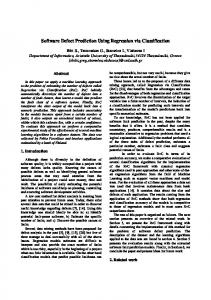
feature and mean of negative ith feature respectively. and indicate ith feature of kpositive and k-negative samples correspondingly. The larger value of F-score indicates that the corresponding feature is more discriminative or highly significant [36, 38-39]. 5.3. Proposed Model Following are the steps of proposed model as shown in Figure 6: Step1: Load the Software defect dataset from PROMISE repository. Step2: Perform pre-processing of the dataset. Step3: Divide the dataset using k-fold cross validation process. Step4: Calculate the F-score for each feature and arrange them in descending order. Step5: Generate new dataset with N features, where N=1,…,m, m is the total number of feature. Step6: Train the model for each feature subset. Step7: Compare the results with different feature subset and with other existing data mining approaches. Step 8: Select the feature subset showing highest accuracy.


49


Figure 6. Proposed Model 5.4. Performance Evaluation Parameters The performance of proposed model is measured with the help of confusion matrix which store the results of classifier in the form of actual and predicted class as indicated in Table 3. Table 3. Confusion Matrix Actual Class

Predicted Class

Defective Not Defective

Defective True Negative (TN) False Negative (FN)

Not Defective False Positive (FP) True Positive (TP)

Performance evaluation model of proposed system is shown in Figure 7.

50



Figure 7. Performance evaluation model for the proposed system Using confusion matrix, we can estimate accuracy, specificity, Precision and F-measure which further utilized for performance evaluation of proposed model [3] a. Accuracy: Accuracy is also referred as “correct classification rate” and is measured by taking the ratio of correctly prediction to the total prediction made by the software defect prediction model and is formulated as: Accuracy= (TP+TN)/(TP+FP+FN+TN)

(22)

b. Sensitivity: Sensitivity, also called true positive rate, is estimated by calculating the % of correctly identified not-defective software modules and is formulated as: Sensitivity= TP/ (TP+FN)

(23)

c. Specificity: Specificity, also termed as true negative rate, is measured by calculating the % of correctly recognized defective modules and is formulated as: Specificity= TN/ (TN+FP)

(24)

d. Precision: Sometime it is also referred as correctness and is measured by taking the proportion of correctly recognized defect free modules and total predicted not-defective software modules by classifier and is formulated as: Precision= TP/(TP+FP)

(25)

e. F-Measure: It is measured by taking the harmonic mean of precision and sensitivity and is calculated as: F-Measure= (2 *Sensitivity*Precision)/ (Sensitivity + Precision)


(26)

51


6. Results and Discussion This paper has performed experiment on 4 PROMISE datasets as CM1, PC1, KC1 and KC2. We also applied normalization technique to all datasets. Normalization has been performed by dividing each attribute value with maximum value of that particular attribute. The F-score value of each feature for CM1, PC1, KC1, KC2 datasets are shown in Table 4. Table 4. Average Feature importance of each feature using k-fold cross validation Feature Number 1 2 3 4 5 6 7 8 9 10 11 12 13 14 15 16 17 18 19 20 21

Average F-score CM1 PC1 0.1699 0.3457 0.1742 0.3096 0.1288 0.2158 0.1156 0.1924 0.1158 0.2276 0.1044 0.2166 0.0465 0.1353 0.0455 0.1023 0.0506 0.0952 0.0364 0.0725 0.0350 0.0726 0.0288 0.0616 0.0246 0.0644 0.0256 0.0694 0.0263 0.0721 0.0293 0.0733 0.0292 0.0746 0.0280 0.0711 0.0270 0.0678 0.0249 0.0657 --0.0601

KC1 0.4067 0.4962 0.3596 0.2964 0.2655 0.2277 0.0839 0.1176 0.1113 0.0848 0.0760 0.0663 0.0675 0.0618 0.0594 0.0706 0.0702 0.0656 0.0621 0.059 ---

KC2 0.0018 0.0025 0.0023 0.0022 0.0020 0.0017 0.0005 0.0007 0.0006 0.0005 0.0004 0.0004 0.0004 0.0004 0.0004 0.0004 0.0005 0.0004 0.0004 0.0004 0.0003

Twenty one predictive models are constructed using different number of feature. Then the LSTSVM model is constructed and learned for each feature set. This study has performed experiment using 10-fold cross validation in windows 7, 64-bit operating system. The performance of each model is evaluated using equation 22-26. The model with better performance is selected and further utilized for defect prediction in software modules. For CM1 dataset the descending order of feature according to its F-score values are- F2, F1, F3, F5, F4, F6 and so on. In the same way, for PC1 dataset the rank of features are F1, F2, F5, F6, F3, F4, F7, F8 and so on according to their F-score. We found that LOC, cyclomatic complexity, essential complexity, design complexity, difficulty and effort measure are significant metrics for defect prediction. Table 5 represents the 21 predictive models having different feature subset for PC1 dataset. In the same way, this study also obtains different predictive models with different number of feature. Then, the performance of each predictive model against different performance estimators is evaluated using 10-fold cross validation method.

52



Table 5. Feature subset Model for PC1 dataset

Performance comparison of PC1, CM1, KC1 and KC2 datasets with different models have compared using accuracy, sensitivity, precision, F-measure and specificity. Table 6, 7, 8 and 9 indicate the comparative analysis of proposed approach using above mentioned parameters against four datasets. Table 6. Performance comparison of PC1 dataset Model #1 #2 #3 #4 #5 #6 #7 #8 #9 #10 #11 #12 #13 #14 #15 #16 #17 #18 #19 #20 #21

Accuracy 94.53% 89.05% 89.88% 90.71% 94.42% 94.63% 94.34% 93.62% 94.06% 91.04% 89.66% 87.61% 86.71% 87.33% 86.89% 86.35% 85.49% 92.40% 92.28% 88.87% 86.65%


Precision 0.9346 0.9523 0.9519 0.9515 0.9383 0.9575 0.9396 0.9440 0.9403 0.9460 0.9468 0.9529 0.9572 0.9545 0.9555 0.9568 0.9444 0.9328 0.9157 0.9545 0.9609

F-measure 0.9612 0.9284 0.9348 0.9396 0.9603 0.9614 0.9587 0.9529 0.9571 0.9411 0.9392 0.9230 0.9271 0.9246 0.9192 0.9121 0.9254 0.9035 0.9017 0.9048 0.8995

Sensitivity 0.9904 0.9064 0.9162 0.9310 0.9835 0.9875 0.9816 0.9663 0.9758 0.9400 0.9265 0.8972 0.8865 0.8950 0.8873 0.8786 0.8685 0.9693 0.9638 0.9077 0.8860

Specificity 0.7639 0.7894 0.7728 0.7061 0.7344 0.7150 0.7428 0.7467 0.8780 0.8294 0.8161 0.8256 0.7428 0.7144 0.7567 0.7678 0.7500 0.8417 0.8667 0.6650 0.6422

53

International Journal of Advanced Science and Technology Vol. x, No. x, xxxxx, 2014

Table 7. Performance comparison of CM1 dataset Model #1 #2 #3 #4 #5 #6 #7 #8 #9 #10 #11 #12 #13 #14 #15 #16 #17 #18 #19 #20

Accuracy 89.16% 88.96% 90.36% 87.95% 87.35% 82.72% 80.33% 79.15% 83.14% 90.45% 70.65% 60.18% 60.37% 58.37% 58.63% 58.42% 65.85% 73.37% 82.37% 81.53%

Precision 0.9423 0.9345 0.9117 0.9342 0.9011 0.9366 0.8643 0.9094 0.8832 0.9507 0.9211 0.8974 0.9101 0.9093 0.8931 0.8887 0.8867 0.9282 0.8981 0.8634

F-measure 0.8981 0.9048 0.9072 0.9003 0.9187 0.8624 0.8802 0.8771 0.9015 0.9376 0.7831 0.7786 0.8771 0.7354 0.7527 0.7372 0.7563 0.7694 0.8993 0.8759

Sensitivity 0.8964 0.9177 0.9256 0.9183 0.9383 0.8758 0.8779 0.8437 0.9147 0.9210 0.6847 0.7902 0.8479 0.6451 0.6841 0.6289 0.6371 0.6944 0.9002 0.9261

Specificity 0.7674 0.7650 0.8311 0.8154 0.8276 0.7963 0.7841 0.6340 0.8407 0.7761 0.7063 0.5474 0.5341 0.4228 0.4276 0.5494 0.7702 0.7582 0.7353 0.7254

Table 8. Performance comparison of KC1 dataset Model #1 #2 #3 #4 #5 #6 #7 #8 #9 #10 #11 #12 #13 #14 #15 #16 #17 #18 #19 #20

54

Accuracy 84.69% 85.39% 85.25% 83.88% 85.06% 70.61% 78.05% 85.15% 86.06% 85.21% 83.07% 82.83% 79.98% 79.07% 71.74% 69.75% 71.60% 73.51% 73.03% 74.46%

Precision 0.8718 0.8680 0.8717 0.8842 0.8811 0.9366 0.9136 0.8908 0.9401 0.8899 0.8987 0.8974 0.9101 0.9093 0.9311 0.8887 0.9340 0.9368 0.9382 0.9391

F-measure 0.9074 0.9125 0.9112 0.9007 0.9087 0.7824 0.8478 0.9111 0.9143 0.9087 0.9001 0.8986 0.8771 0.8754 0.7827 0.7572 0.7652 0.7730 0.7684 0.7631

Sensitivity 0.9462 0.9619 0.9456 0.9181 0.9383 0.6758 0.7930 0.9327 0.9417 0.9288 0.9024 0.9002 0.8479 0.8451 0.7841 0.6371 0.6527 0.6617 0.6544 0.6466

Specificity 0.6392 0.6991 0.6299 0.6407 0.6067 0.7427 0.5825 0.6710 0.6527 0.6680 0.6386 0.6353 0.6370 0.6340 0.7050 0.7702 0.7400 0.7491 0.7582 0.7642


Table 9. Performance comparison of KC2 dataset Model #1 #2 #3 #4 #5 #6 #7 #8 #9 #10 #11 #12 #13 #14 #15 #16 #17 #18 #19 #20 #21

Accuracy 82.47% 85.13% 85.7% 85.89% 85.89% 86.07% 86.04% 85.54% 86.12% 84.72% 83.9% 83.13% 82.77% 83.03% 81.83% 81.81% 81.26% 81.39% 80.41% 79.37% 79.86%

Precision 0.8100 0.8297 0.8418 0.8446 0.8667 0.8605 0.8584 0.8679 0.8939 0.8534 0.8591 0.8525 0.8728 0.8735 0.8693 0.8606 0.8681 0.8779 0.8662 0.8933 0.8937

F-measure 0.8943 0.9022 0.9081 0.9089 0.9118 0.9086 0.9049 0.8947 0.8907 0.8998 0.9018 0.9028 0.8870 0.8827 0.8671 0.8678 0.8739 0.8822 0.8802 0.8694 0.8752

Sensitivity 1.0000 0.9842 0.9836 0.9814 0.954 0.9654 0.9584 0.9289 0.9405 0.9624 0.9671 0.9624 0.9318 0.9321 0.9226 0.9181 0.9367 0.9173 0.8775 0.8575 0.8507

Specificity 0.4642 0.6047 0.6505 0.6667 0.6837 0.6528 0.6607 0.7782 0.7142 0.6176 0.6716 0.6389 0.7120 0.7020 0.7145 0.7199 0.7199 0.7707 0.7838 0.6023 0.6026

It is clear from the above results that model-10 of CM1, model -6 of PC1, model- 9 of KC1 and KC2 dataset has performed well in terms of accuracy, precision and F-measure. The accuracy of model-6 of PC1 is 94.63%, precision is 95.75 % and F-measure is 96.14 % while the above mentioned parameters for model-10 of CM1 dataset are 90.45%, 95.07% and 93.76% respectively. Accuracy, Precision and F-measure for model-9 of KC1 and KC2 dataset are 86.06%, 94.01%, 91.43% and 86.12%, 89.39%, 89.07% respectively. Performance of proposed model for sensitivity and specificity against above stated datasets varies from one model to another. So considering sensitivity and specificity as a performance measure is not making any sense, thus this research work considers accuracy, precision and F-measure to evaluate the performance of classifier. This study also performed a comparative analysis of feature selection based LSTSVM model with other existing methods. Comparative analysis of various classification approaches against four PROMISE datasets is shown in table 10. The proposed feature selection based LSTSVM predictive model for software defect prediction performs well with PC1, KC1 and KC2 dataset. Accuracy of proposed approach for CM1 dataset is also comparable with SVM.

55


Table 10. Comparative analysis with other existing dataset Prediction Approach This study SVM LR KNN MLP RBF BBN DT

CM1 90.45% 90.69% 90.17% 83.27% 89.32% 89.91% 76.83% 89.82%

PC1 94.63% 93.10% 93.19% 91.82% 93.59% 92.84% 90.44% 93.58%

KC1 86.06% 84.59% 85.55% 83.99% 85.68% 84.81% 75.99% 84.56%

KC2 86.12% 84.67% 82.90% 81.19% 84.48% 83.57% 82.80% 82.85%

7. Conclusion This study proposed a feature selection based LSTSVM model for defect prediction. Fscore feature selection technique is used to select significant feature which are helpful to predict defects in software modules. There is a significant difference in classifier’s performance which is developed using new feature subset as compared to the classifier built on complete feature set. This study has evaluated the predicting performance of proposed model for defective software modules and also performed a comparative analysis against seven statistical and machine learning approaches using four PROMISE datasets. The experimental results show that the predictive capability of the proposed approach is better or at least comparable with other approaches. This research discloses the effectiveness of proposed feature selection based LSTSVM approach in predicting defective software modules and suggests that the proposed model can be useful in predicting software quality. The performance of proposed work can also be compared by using other feature selection techniques as well as other software repositories so that the impact of changing the feature selection method, datasets in LSTSVM could also be established.

References [1] N. E. Fenton and S. L. Pfleeger, “Software metrics: a rigorous and practical approach”, PWS Publishing Co., (1998). [2] A. Koru and H. Liu, “Building effective defect-prediction models in practice”, IEEE Software, (2005), pp. 23–29. [3] A. Sonali and D. Siddhant, “Prediction of Software Defects using Twin Support Vector Machine”, 2nd International conference on Information Systems & computer Networks (ISCON-2014), In press. [4] A. Okutan O. T. Yıldız, “Software defect prediction using Bayesian networks”, Empirical Software Engineering, (2012), pp. 1-28. [5] K. O. Elish and M. O. Elish, “Predicting defect-prone software modules using support vector machines”, The Journal of Systems and Software, vol. 81, (2008), pp. 649–660. [6] Y. Hu, X. Zhang, X. Sun, M. Liu and J. Du, “An intelligent model for software project risk prediction”, In: International conference on information management, innovation management and industrial engineering, vol. 1, (2009), pp. 629–632. [7] C. Jin and J. Liu, “Applications of support vector machine and unsupervised learning for predicting maintainability using object-oriented metrics”, 2010 second international conference on multimedia and information technology (MMIT), vol. 1, (2010), pp. 24–27. [8] Q. Song, M. Shepperd, M. Cartwright and C. Mair, “Software defect association mining and defect correction effort prediction”, IEEE Trans Softw Eng., vol. 32, no. 2, (2006), pp. 69–82. [9] G. Boetticher, T. Menzies and T. Ostrand, “Promise repository of empirical software engineering data”, Department of Computer Science, West Virginia, University, (2007), http://promisedata.org/repository. [10] N. Fenton, M. Neil and D. Marquez, “Using Bayesian networks to predict software defects and reliability”, J Risk Reliability, vol. 222, no. 4, (2008), pp. 701–712. [11] D. Zhang, “Applying machine learning algorithms in software development”, Proceedings of the 2000 Monterey workshop on modeling software system structures in a fastly moving scenario, (2000), pp. 275–291.

56


[12] R. Jayadeva, R. Khemchandani and S. Chandra, “Twin Support vector Machine for pattern classification”, IEEE Trans Pattern Anal Mach Intell., vol. 29, no. 5, (2007), pp. 905-910. [13] V. Basili, L. Briand and W. Melo, “A validation of object-oriented design metrics as quality indicators”, IEEE Transactions on Software Engineering, vol. 22, no. 10, (1996), pp. 751–761. [14] S. Henry and D. Kafura, “The evaluation of software systems' structure using quantitative software metrics”, Software: Practice and Experience, vol. 14, no. 6, (1984), pp. 561-573. [15] M. A. Cusumano, “Japan’s Software Factories”, Oxford University Press, (1991). [16] L. Guo, Y. Ma, B. Cukic and H. Singh, “Robust prediction of fault proneness by random forests”, Proceedings of the 15th International Symposium on Software Reliability Engineering (ISSRE’04), (2004), pp. 417–428. [17] H. A. Al-Jamimi and L. Ghouti, “Efficient prediction of software fault proneness modules using support vertor machines and probabilistic neural networks”, IEEE, 5th Malaysian Conference in Software Engineering (MySEC), (2011)B. [18] T. Khoshgoftaar, E. Allen, J. Hudepohl and S. Aud, “Application of neural networks to software quality modeling of a very large telecommunications system”, IEEE Transactions on Neural Networks, vol. 8, no. 4, (1997), pp. 902–909. [19] J. Kaur and Pallavi, “Data Mining Techniques for Software Defect Prediction”, International Journal of Software and Web Sciences (IJSWS), (2013), pp. 54-57. [20] Z. Yan, X. Chen and P. Guo, “Software Defect Prediction Using Fuzzy Support Vector Regression”, Springer-Verlag Berlin Heidelberg, (2010). [21] H. Can, X. Jianchun, Z. R. L. Juelong, Y. Quiliang and X. Liqiang, “A new model for software defect prediction using particle swarm optimization and support vector machine”, IEEE, (2013). [22] D. Hand, H. Mannila and P. Smyth, “Principles of data mining”, MIT, (2001). [23] J. Han and M. Kamber, “Data mining: concepts and techniques”, 2nd ed. The Morgan Kaufmann Series, (2006). [24] T. Divya and A. Sonali, “A survey on Data Mining approaches for Healthcare”, International Journal of BioScience and Bio-Technology, vol. 5, no. 5, (2013), pp. 241-266. [25] N. Gayatri, S. Nickolas and A. V. Reddy, “Feature selection using decision tree induction in class level metrics dataset for software defect predictions”, In Proceedings of the World Congress on Engineering and Computer Science, vol. 1, (2010), pp. 124-129. [26] J. Wang, B. Shen and Y. Chen, “Compressed C4. 5 Models for Software Defect Prediction”, 2012 12th International Conference on Quality Software (QSIC), IEEE, (2012) August, pp. 13-16. [27] J. Zheng, “Cost-sensitive boosting neural networks for software defect prediction”, Expert Systems with Applications, vol. 37, no. 6, (2010), pp. 4537-4543. [28] C. Cortes and V. Vapnik, “Support Vector Network”, Mach Learn., vol. 20, (1995), pp. 273-297. [29] V. Vapnik, “The nature of statistical Learning, @nd edn”, Springer, New York, (1998). [30] N. Chistianini and J. Shawe-Taylor, “An Introduction to Support Vector Machines, and other kernel-based learning methods”, Cambridge University Press, (2000). [31] N. Cristianini and J. Shawe-Taylor, “An Introduction to Support Vector Machines”, Cambridge University Press, (2000). [32] T. G. Dietterich and G. Bakiri, “Solving multiclass learning problems via error-correcting output codes”, Journal of Artificial Intelligence Research, vol. 2, (1995), pp. 263–286. [33] B. Sch¨olkopf, C. Burges and A. Smola, (Eds.), “Advances in Kernel Methods—Support Vector Learning”, MIT Press, (1998). [34] C. W. Hsu, C. C. Chang and C. J. Lin, “A practical guide to support vector classification”, http://www.csie.ntu.edu.tw/~cjlin/papers/guide/guide.pdf, (2003). [35] M. A. Kumar and M. Gopal, “Least squares twin support vector machines for pattern classiﬁcation”, Expert Systems with Applications, vol. 36, (2009), pp. 7535–7543. [36] T. Divya and A. Sonali, “Feature Selection based Least Square Twin Support Vector Machine for diagnosis of heart disease”, Unpublished Manuscript. [37] Software Defect Dataset, PROMISE REPOSITORY, http://promise.site.uottawa.ca/SERepository/datasetspage.html, (2013) December 4. [38] Y. W. Chen and C. J. Lin, “Combining SVMs with various feature selection strategies”, http://www.csie.ntu.edu.tw/~cjlin/ papers/features.pdf, (2005). [39] M. F. Akay, “Support vector machines combined with feature selection for breast cancer diagnosis”, Expert systems with applications, vol. 36, no. 2, (2009), pp. 3240-3247.

57


Authors Dr. Sonali Agarwal Dr. Sonali Agarwal is working as an Assistant Professor in the Information Technology Division of Indian Institute of Information Technology (IIIT), Allahabad, India. Her primary research interests are in the areas of Data Mining, Data Warehousing, E Governance and Software Engineering. Her current focus in the last few years is on the research issues in Data Mining application especially in E Governance and Healthcare.

Divya Tomar She is a research scholar in Information Technology Division of Indian Institute of Information Technology (IIIT), Allahabad, India under the supervision of Dr. Sonali Agarwal. Her primary research interests are Data Mining, Data Warehousing especially with the application in the area of Medical Healthcare.

58