Automatic Feature Selection for Model-Based Reinforcement Learning

Automatic Feature Selection for Model-Based Reinforcement Learning in Factored MDPs Mark Kroon and Shimon Whiteson Informatics Institute, University of Amsterdam, Science Park 107, 1098 XG Amsterdam The Netherlands {m.kroon,s.a.whiteson}@uva.nl

Abstract—Feature selection is an important challenge in machine learning. Unfortunately, most methods for automating feature selection are designed for supervised learning tasks and are thus either inapplicable or impractical for reinforcement learning. This paper presents a new approach to feature selection specifically designed for the challenges of reinforcement learning. In our method, the agent learns a model, represented as a dynamic Bayesian network, of a factored Markov decision process, deduces a minimal feature set from this network, and efficiently computes a policy on this feature set using dynamic programming methods. Experiments in a stock-trading benchmark task demonstrate that this approach can reliably deduce minimal feature sets and that doing so can substantially improve performance and reduce the computational expense of planning. Keywords-Reinforcement learning; feature selection; factored MDPs

I. I NTRODUCTION In many machine learning problems, the set of features with which the data can be described is quite large. Feature selection is the process of determining which subset of these features should be included in order to generate the best performance. Doing so correctly can be critical to the success of the learner. Clearly, excluding important features can limit the quality of the resulting solution. At the same time, including superfluous features can lead to slower learning or weaker final performance, since the number of potential solutions grows exponentially with respect to the number of features. In addition, using a non-minimal feature set may incur other costs, e.g., the expense of purchasing and installing unnecessary sensors on a robot. This paper considers the problem of feature selection in reinforcement learning (RL) problems [1], in which an agent seeks a control policy for an unknown environment given only a scalar reward signal as feedback. The need for methods that automate feature selection in RL is great, as most existing feature selection methods assume a supervised setting, in which the goal is to approximate a function given example input-output pairs. As a result, they cannot be directly applied to RL problems. For example, filter methods [2], [3] rely on the examples’ labels, which are not available in RL, to filter out irrelevant features as a preprocessing step. Wrapper methods [4], [5], which conduct a ‘meta-search’ for feature sets that maximize the learner’s

performance, do not use labeled data but are nonetheless impractical in RL since the cost of evaluating candidate feature sets affects not just the computational complexity but also the sample complexity [6], i.e., the number of interactions with the environment required for learning. Since RL methods are typically evaluated in an on-line setting, minimizing sample complexity is essential to performance. In this paper, we propose a new approach to feature selection designed to achieve greater sample efficiency. To do so, we employ a model-based [7], [8] approach, wherein the samples gathered by the agent are used to approximate a model of the environment from which a policy is computed using planning methods such as dynamic programming. Assuming the problem is a factored Markov decision process (MDP), this model can be represented as a dynamic Bayesian network (DBN) that describes rewards and state transitions as a stochastic function of the agent’s current state and action. The main idea is to use the conditional independencies shown in such a DBN, whose structure and weights can be learned with recently developed methods [9], [10], to deduce the minimal feature set. In particular, we propose and compare several ways to use the DBN to compute a feature set that not only excludes irrelevant features but also minimizes the size of the feature set in cases when multiple DBNs are consistent with the data. We study the performance of this method in several variations of the stock-trading domain [9]. First, we assess the ability of the method to deduce the right feature set assuming a correct model has already been learned. Then, we consider the performance of the complete algorithm in two RL settings where feature selection can be beneficial. The results show that the proposed method can reliably deduce minimal feature sets and that doing so can substantially improve performance and reduce the computational expense of planning. II. R EINFORCEMENT L EARNING IN FACTORED MDP S A Markov decision process (MDP) can be defined as a 5tuple S, A, T, R, γ, where S is a finite set of states, A is a finite set of actions and T is a transition model T : S × A → PS where PS is a probability distribution over S. T (s |s, a) denotes the probability of transitioning to state s after taking action a in state s. R is a reward function R : S × A → R and γ is a discount factor on the summed sequence of rewards.

The agent’s behavior is determined by its policy π : S → A, which has an associated value function V π : S → R representing the expected discounted future reward starting from a given state and following π. The optimal policy π ∗ can be derived from the optimal value function V ∗ . In a modelbased approach to RL [7], [8], first a model is learned from the environment (i.e., T and R) and then the optimal value function can be computed using a planning technique like value iteration [11]. Some model-based methods, such as the Rmax algorithm [12], are guaranteed to find a near-optimal policy in polynomial time. Rmax ensures efficient exploration of the environment by distinguishing between states that have been visited often enough to accurately estimate the transition function (i.e., they are marked as “known”) and those that have not. The algorithm guides the agent towards unknown states by giving transitions to them an artificial bonus value in the model. Planning on this model then yields a policy that favors exploration in those unknown states. In many MDPs, the state space is spanned by a number of factors X = {X1 , · · · , Xn }, where each factor Xi takes on values in some finite domain D(Xi ). In a factored MDP, each state s ∈ S is represented as a vector s = s(1), · · · , s(n), where s(i) ∈ D(Xi ). The number of states grows exponentially in the number of factors. If not all factors of a state influence all factors at the next timestep, the transition function can be represented succinctly with a dynamic Bayesian network (DBN) [13]. In a typical formulation, there is one DBN for each action a ∈ A. Each DBN consists of a two-layer graph in which the layers represent the states at time t and t + 1. The nodes in the graph represent factors and the edges denote dependency relations given the action a. P aa (Xi ) denotes the parents of the ith factor for action a, the set of factors in the previous timestep that directly influence this particular factor. As in previous literature [14], [15], [9], we assume that a factor Xi at time t+1 is conditionally independent of all other factors at time t + 1 given the factors at time t. The transition function can now be described as:  Pi (s (i)|ui , a) T (s |s, a) =

KWIK learner. The resulting method, which we call KWIKFactored-Rmax, is shown in Algorithm 1. Here, the KWIK model learner K is an implementation of the outline made by Li et al., and is comparable with the recent Met-Rmax implementation introduced by Diuk et al. [17]. K is instantiated with accuracy parameters  and δ and learns a model from samples of the form s, a, r, s  obtained by the agent. Specifically, it learns both the structure and CPT entries of DBNs for the transition and reward functions. When queried for a prediction, K(s, a) may return ⊥ if it has not observed enough examples to estimate the reward or next state resulting from taking action a in state s. Otherwise, it returns Tˆ(s |s, a), an estimate of the transition function ˆ a), an estimate of the reward function such that and R(s,  ˆ a) − R(s, a)| ≤ , ˆ |T (s |s, a) − T (s |s, a)| ≤  and |R(s, both with probability 1 − δ. Internally, the algorithm learns a dependency structure for each feature Xi separately by considering different hypothetical parent sets P aa (Xi ) with up to k parent nodes. The parent sets that result in high prediction errors are discarded. We refer to [10] for more details about KWIK learning. Algorithm 1 KWIK-Factored-Rmax(, δ, θ) Inputs: , δ: accuracy thresholds for the KWIK model learner θ: accuracy threshold for value iteration Initialize KWIK model learner K with parameters  and δ. for all (s, a) ∈ S × A do Q(s, a) ← Rmax // initialize action-value function for each timestep t do Let s denote the state at t. Take action a = arg maxa ∈A Q(s, a ). Let s be the next state after taking action a in state s. Let K observe s, a, r, s . repeat Δ←0 for all (s, a) ∈ S × A do if K(s, a) = ⊥ then Q(s, a) ← Rmax else // otherwise perform value iteration update ˆ ← K(s, a) Tˆ , R v ← Q(s, a)     ˆ Tˆ (s |s, a) max Q(s , a ) Q(s, a) ← R(s, a) + γ s

a

Δ ← max(Δ, |v − Q(s, a)|) until Δ < θ

i

where ui is the setting of the factors in P aa (Xi ) and Pi (·|ui , a) is a probability distribution over D(Xi ) defined by a conditional probability table (CPT). The extension to represent the reward function is straightforward. Existing approaches to learn factored MDPs such as Factored-Rmax [16] assume the structure of the model to be known and only learn the CPTs. However, recently proposed algorithms can also learn the structure of the model [9], [10]. Li et al. [10] introduce the knows what it knows (KWIK) framework and outline a KWIK-algorithm to learn structure and parameters for a factored MDP. Since a KWIK learner can respond to queries with ⊥ (meaning “I don’t know”), it can be naturally integrated with Factored-Rmax by giving bonus rewards to transitions from states labeled unknown by the

III. T HE F EATURE S ELECTION P ROBLEM FOR RL The goal of feature selection is to improve the learner’s speed and/or performance by removing irrelevant and redundant features. In this paper, we consider two settings in which automatic feature selection can be beneficial to an RL agent. First, we consider a setting involving transfer learning [18], [19], in which the agent strives to exploit its experience on a source task to learn more efficiently on a related target task. Transfer is possible because of some prior knowledge about the relationship between the two tasks. In our case, we assume that the tasks share the same minimal set of features, and thus the results of feature selection performed on the source task can be transferred to the target task in order to speed up learning and improve performance. This is a

natural assumption because, in many real-world scenarios, the usefulness of certain features is fixed across related tasks. One example is the stock-trading domain considered in this paper, where market dynamics can shift over time, but which stock characteristics are relevant remains fixed. Another example is robot navigation, where the locations of obstacles can change from one building to another but the sensors needed to detect them may be the same. We focus on a typical scenario considered during evaluation of transfer learning methods. Following Taylor et al. [18], we call this the total time scenario1 in which learning occurs on the source task for the sole purpose of gleaning information useful for improving performance on the target task. Improving performance in this scenario is challenging because the costs of learning the source task have to be considered during evaluation. The other setting we consider consists of the traditional RL problem of learning a policy on-line in a single, fixed task. This setting is even more challenging because there is no opportunity for transfer. Instead, feature selection is beneficial only if the correct features can be identified early enough to substantially speed further learning on the same task. Existing approaches for feature selection in RL problems includes the FS-NEAT method [20], which takes a modelfree approach. This contrasts with our approach, which uses a model learned from data and thus addresses the complication that multiple DBNs may be consistent with the data (see Section IV-A). Another related approach is the SCRAM-Rmax algorithm by Diuk et al. [17] which uses the KWIK framework to compare classifiers based on different feature subsets. They assume however, the maximum number of potentially relevant features is provided, while we are concerned with finding the optimal size of the feature set. Feature selection as described here is also related to the problem of automating the choice of basis functions for value function approximation in RL, for which novel methods have recently been developed. For example, Mahadevan and Maggioni [21] propose an algorithm that learns an undirected graph of the environment and uses it to find a set of basis functions for compactly approximating the value function. Because the method generates the basis functions instead of just choosing among them, it is more akin to feature construction [22], [23] than feature selection. Another related method is that of Parr et al. [24] who propose to iteratively add basis functions to a linear approximation architecture based on their ability to reduce Bellman error. Like the work of Mahadevan and Maggioni, this method focuses on finding basis functions that yield the lowest error in value function approximation, whereas the goal of our work is to find a minimal feature set that still allows exact representation of the optimal value function. Feature selection is also closely related to state abstraction, where the goal is to identify groups of states that can be 1 We use this terminology to be consistent with Taylor et al. [18], wherein ‘time’ refers to sample complexity. However, our experiments also evaluate computational costs.

treated as one. State abstraction typically focuses on contextspecific independence, (i.e., whether a feature can be ignored is conditional on the value of other features). This contrasts with feature selection, which seeks features that can be ignored in every state. While context-specific independence is more powerful, it can be computationally intractable [25] or require making more restrictive assumptions [26]. Methods for state abstraction typically learn in a model-free way [27] or plan assuming a model is given [25], [26]. Again, this contrasts with our model-based approach wherein the model is learned from data. IV. M ODEL -BASED F EATURE S ELECTION FOR RL The main idea of our approach is to use the conditional independencies shown in the DBN model of a factored MDP to deduce the correct feature set. As noted by Parr et al. [28], a relevant feature for reinforcement learning is one that helps predict the immediate reward or next state the agent will experience. However, features that help to predict the next state may still be irrelevant because, while they are the parents of some state features, those features themselves may be irrelevant. Hence, we employ a stricter condition, namely that each feature in the set must, directly or indirectly, help predict reward. As Boutilier and Dearden [29] point out, this can be expressed as a recursive definition: a feature is relevant if it helps predict reward or helps predict a relevant feature. An implementation of an algorithm that generates a feature set according to this definition is outlined in Algorithm 2, it is named FeatureExtraction because it “extracts” the feature set from DBN structures. Algorithm 2 FeatureExtraction(D) Inputs: D (DBN structures defining P aa (Xi ) relations for all actions a ∈ A and features Xi ∈ X) Let X be the original set of features. Let A be the set of actions. S ← set of all Xi ∈ X that directly influence reward repeat S ← ∅ for all Xi ∈ S do for all Xj ∈ X do for all a ∈ A do if Xj ∈ P aa (Xi ) ∧ Xj ∈ / S then S  ← S  ∪ Xj S ← S ∪ S until S  = ∅ return S

A. Feature Selection with Multiple DBNs The FeatureExtraction algorithm is only useful for detecting relevant features when there is just one DBN for each action. However, in practice, the KWIK model learner often returns multiple DBNs, as more than one DBN structure may be consistent with the available data. This can occur because the KWIK learner has no mechanism to favor parsimonious models; thus, it discards structures that are missing necessary edges but not those containing superfluous edges. Multiple DBNs can also be returned if the full feature set contains redundant

features. For example, suppose that for action a1 , X1 and X2 contain the same information, which directly influences X3 . Then, a valid DBN could have either X1 ∈ P aa1 (X3 ) or X2 ∈ P aa1 (X3 ). The presence of multiple consistent DBNs for each action is a potential problem for feature selection. If the agent selects a DBN for each action arbitrarily, then the feature set produced by the FeatureExtraction algorithm may be not be minimal. For example, suppose that action a2 has the same dependencies as a1 in the example above. If the agent uses a DBN for a1 wherein X1 ∈ P aa1 (X3 ) but for a2 uses a DBN wherein X2 ∈ P aa2 (X3 ), then the resulting feature set will include both X1 and X2 even though only one of them is necessary. The problem the agent faces is to find the set of DBNs, one for each action, that results in a minimal feature set when used as input to the FeatureExtraction algorithm. Unfortunately, the number of possible DBN structures for each action grows exponentially with respect to the number of features. We propose and compare several approaches to searching for the best set of DBNs to use in feature selection. The first method, ExhaustiveSearch, simply iterates through all possible combinations, running the FeatureExtraction algorithm on each of them. Finally, it returns a configuration for which the resulting feature set is the smallest. This method guarantees to find the minimal feature set given the model produced by the KWIK learner, but will be computationally infeasible except in problems with few features. The second method, UnionOfMinimums, selects the minimal DBN for each action, i.e., the DBN with the fewest edges. Here, the number of edges is used as a heuristic to minimize the number of connections from features to reward. Since the DBN for each action is selected individually, without consideration of the DBNs selected for the other actions, there is no guarantee that the resulting feature set will be minimal. However, the method is much more computationally efficient, as the FeatureExtraction algorithm needs to be run only once. The third method, GreedySearch, builds a DBN for each action using parent sets returned by the KWIK learner as building blocks. For each action, the KWIK learner usually provides multiple parent sets P a(Xi ) for each feature Xi . The GreedySearch method starts by ordering the features for all actions by the size of their smallest parent set. Beginning with the feature and action for which the smallest parent set is greatest, this smallest parent set is used as a first building block to construct a DBN for the current action. The method then iterates over all features for all actions and uses the parent set for the construction of the DBNs such that the size of the resulting feature set generated by the FeatureExtraction algorithm applied to those rudimentary DBNs is minimized. The set of DBNs constructed by the GreedySearch method may be suboptimal because at each iteration, a parent set is chosen without consideration of features and their parent sets visited in later iterations. The fourth method, HillClimbing, begins by randomly selecting a parent set, from among those returned by the KWIK model learner, for all features for each action. It constructs a

set of DBNs from this collection of parent sets. Subsequently, it tries to minimize the size of the feature set generated by the FeatureExtraction algorithm by locally changing the configuration, i.e., by switching only the parent set for one feature for one action at the time. When there is no more improvement possible by doing these local changes, the method terminates. The feature selection methods described above can be integrated with KWIK-Factored-Rmax to produce a complete RL algorithm. However, in the on-line setting, KWIK-FactoredRmax has to be augmented to decide when it has learned the model well enough to run the feature selection method. If it is done too early, the model may still be inaccurate, leading to incorrect feature selection and suboptimal asymptotic performance. If it is done too late, the agent may already have found such a good policy from planning with the full feature set that no benefit occurs. To balance these factors, we introduce a threshold parameter τ on the model accuracy. We measure model accuracy as the ratio of accurate predictions by the KWIK model learner to the number of ⊥’s. While the number of accurate predictions divided by the number of ⊥’s is below this threshold, the agent uses KWIK-Factored-Rmax with the full feature set. When this value reaches τ , the agent performs feature selection using the current model and then continues to apply KWIK-Factored-Rmax with the reduced feature set. V. S TOCK T RADING D OMAIN To evaluate our methods, we employ the stock-trading domain that has been used in earlier research on factored MDPs [9], [17]. This domain is an appropriate choice because we know from previous results that it is feasible for current methods to learn a factored model in it and because it can be naturally augmented to present a feature selection challenge. The stock-trading domain consists of a number of stocks grouped into several sectors. The stock values are either rising or falling. An agent can buy or sell all stocks of one whole sector at a time or do nothing. At each timestep, for all stocks in sectors that it owns, the agent receives a reward of +1 when the stock is rising and −1 when the stock is falling. Whether a stock is rising or falling depends on the number of stocks that were rising in the same sector in the previous timestep. An agent performs well when it is able to predict future stock values and make sure to own sectors at times they have many stocks rising. We augment the stock-trading domain in two ways. First, we add a number of global economic features that affect the value of all stocks. Specifically, such a global economic feature is binary and when it has a value of 1, it increases the probability of a stock to be rising at the next timestep, the stock value is negatively influenced when the economic variable has a value of 0. These features are introduced to create indirect influences on reward, thus testing the ability of our method to find indirectly relevant features. Second, we add irrelevant and redundant features to make feature selection potentially beneficial. A particular problem in the stock-trading domain can be formalized as st(E, O, U, I, V ) where E is the number of

1.5

1

0.5

0

P (stock rising) = 0.1 + 0.8 ×

#stocks in sector rising

(1)

+ #global economic variables valued 1 + #global economic variables

#stocks in sector

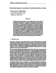
Furthermore, there are I features that represent irrelevant information sources whose value is randomly chosen at every timestep. Finally, there are V redundant features that are copies of a relevant feature of the same problem, randomly chosen at the beginning of each experimental run. The DBN structure for the reward function R(s, a) consists of E + E × O + U edges from the stocks and global economic features to the reward. To lower the burden on the structure learner, we describe the total reward as the sum of E × O subrewards, each representing the reward received for a single stock. While a sub-reward depends on O + U + 1 features, using all of them would eliminate the presence of indirectly relevant features. Therefore, during learning we limit the maximum degree of the DBN of a sub-reward to O + 1. As a result, sub-rewards are not perfectly learnable but, as the experiments in the next section show, good policies are nonetheless discovered. VI. E XPERIMENTAL R ESULTS In all experiments, we average the results over 10 runs and k, the maximum in-degree of the DBN structures learned by the KWIK-Factored-Rmax algorithm is assumed to be known. In a first experiment, we compare the quality of the feature sets selected by each of the four methods introduced in Section IV-A in the case where an accurate model has already been learned. In each run, we use KWIK-FactoredRmax to learn an accurate model (with  = 0.15, δ = 0.15 and τ = 12 ) and then provide that model as input to the feature selector. Precision and recall measures are computed by treating selected unnecessary features as false positives and discarded necessary features as false negatives. Figure 1 shows the results of this experiment on the three stock-trading problems: A = st(1, 1, 1, 1, 1), B = st(1, 2, 1, 1, 1) and C = st(2, 1, 1, 1, 1). The performance of ExhaustiveSearch is shown only for problem A because it was unable to complete in reasonable time on the larger problems. All four methods achieved optimal or near-optimal recall. However, the graph shows that both the MinimumOfUnions and HillClimbing methods have poor precision due to the frequent inclusion of redundant features. Irrelevant features were correctly discarded with just a few exceptions. Both ExhaustiveSearch and GreedySearch achieve optimal precision

UnionOfMinimums HillClimbing GreedySearch ExhaustiveSearch

Precision

sectors, O is the number of stocks per sector, U is the number of global economic features, I is the number of irrelevant features and V is the number of redundant features. A state is represented by E + EO + U + I + V binary features. E features indicate whether the agent owns a particular sector, EO features represent stocks that are either rising or falling, there are U global economic features having no particular meaning except their influence on the stocks. Whether a particular stock is rising is determined by:

A

B Problem

C

Precision for the four feature selection methods on three different stock trading problems.

Fig. 1.

on all three problems, though the latter is much more computationally efficient. Therefore, we use the GreedySearch method in all following experiments. A. Transfer Learning Results In a transfer learning setting, we use KWIK-FactoredRmax (with parameters  = 0.15, δ = 0.15, τ = 16 ) and GreedySearch to find a feature set for the source task. As described in Section III, we assume that the correct feature set is the same in the source and target task. In this particular transfer learning scenario, the costs of learning in both the source and target task must be considered in the evaluation. Successful transfer in this setting is only feasible if the source task is substantially easier than the target task. Otherwise, the cost of learning the source task will likely be greater than the savings achieved by transfer. In the setup, both the source and target task are defined as the stock-trading problem st(1, 3, 0, 1, 1). In this case, the source task differs structurally from the target task. In the source task, whether a stock is rising depends only on that stock in the previous timestep instead of on all stocks in the same sector. The probability that a stock is rising is 0.9 if it was rising at the previous timestep and 0.1 otherwise. Note that this structural change lowers the degree of the DBN network of the source task model from 3 to 1, this reduces the complexity of learning the DBN substantially. For simplicity, we also assume the reward structure is known. Figure 2 shows the performance of the KWIK-FactoredRmax algorithm on the target task using either the selected feature set or the original feature set, each averaged over 10 runs. The performance of both algorithms is shown in the cumulative reward graph. The line representing the algorithm using the selected feature set does not start at the origin but at a later point (indicated with an ‘x’ on the horizontal axis) to account for the average number of steps needed to solve the source task. However, even with this late start, the algorithm that uses the transferred feature set finds a good policy faster and thereby accrues more cumulative reward. Figure 2 also shows the computational costs, measured as the number of queries to the model. In this experiment and the one reported below, we do not include the computational costs of finding a feature set via the GreedySearch algorithm because these

20000

20000

Original Feature Set Selected Feature Set

15000 Cumulative reward

Cumulative reward

15000 10000

10000

5000 0 0 1.0

X 20000

5000 0

40000

60000

Number of steps

80000

100000

0 3.5

Original Feature Set Selected Feature Set

3.0

0.8

20000

X X 40000

X

60000

Number of steps

80000

100000

Late FS No FS Intermediate FS Early FS

Model consultations

Model consultations

2.5

0.6

2.0 1.5

0.4

1.0

0.2 0.00

Late FS No FS Intermediate FS Early FS

0.5 20000

40000

60000

Number of steps

80000

100000

Cumulative reward (top) and cumulative computational cost (bottom) on each timestep of the target task for two algorithms in the total time scenario.

Fig. 2.

costs are negligible.2 The selected feature set starts off with a higher value to account for the average computational cost of solving the source task. The cost of using the original feature set grows much faster, however, and the lines intersect well before a good policy has been found by either algorithm. These results demonstrate that feature selection can be beneficial in transfer learning, as it substantially improves performance and reduces computational costs. B. On-Line Learning Results We also evaluate our feature selection method in an online learning setting. As mentioned in Section III, this is a more challenging setting, since selecting features too early may result in a suboptimal feature set and poor performance while selecting features too late may yield no benefit over using the full feature set. To demonstrate this, we apply 2 For example, in a separate experiment on st(1,1,1,1,1), we found that planning on a single step was 92 times as computationally expensive as GreedySearch.

0.00

20000

40000

60000

Number of steps

80000

100000

Cumulative reward (top) and cumulative computational cost (bottom) on each timestep in the on-line learning setting.

Fig. 3.

KWIK-Factored-Rmax ( = 0.15, δ = 0.15) to the stocktrading problem st(2, 1, 1, 1, 1) and use GreedySearch to select 1 1 1 , 64 , 18 }. We features at some point determined by τ ∈ { 120 refer to these values of τ as early, intermediate, and late feature selection. Figure 3 compares the performance of these three settings to that of KWIK-Factored-Rmax without feature selection, with each method averaged over 10 runs. In the cumulative reward graph, the points at which feature selection occur are denoted with an ‘x’ on the horizontal axis. As expected, late feature selection shows no performance improvement over learning without feature selection. Doing early feature selection results in an inferior policy and less cumulative reward in the long run. The performance of intermediate feature selection shows that, with an appropriate choice of τ , it is possible to get a small performance advantage even in the on-line setting. The computational costs are also presented in Figure 3. Naturally, all algorithms are equally costly initially, as they are planning with the full feature set. However, the costs of planning are reduced when feature selection occurs, resulting in the

sudden changes in slope seen in the graph. Not surprisingly, the earlier feature selection is applied, the greater the computational savings. We see that while improving performance in the on-line setting is quite difficult, reducing computational costs is not, as even late feature selection is computationally cheaper than no feature selection at all. These results also show how τ controls a trade-off between performance and computational costs, as early feature selection results in greater computational savings but worse performance. Nonetheless, with an appropriate value of τ it is possible to obtain both a marginal performance boost and substantial computational savings even in the on-line setting. VII. D ISCUSSION & F UTURE W ORK The results presented above demonstrate 1) that the proposed feature selection method can reliably find a minimal feature set, 2) that it can substantially improve performance and reduce computational costs in transfer learning, and 3) that it can marginally improve performance and substantially reduce computational costs in an on-line setting. We suspect that obtaining larger performance benefits in the on-line setting would be quite difficult. The fundamental problem is that, in an unknown environment, the agent must explore with respect to all the available features to determine their relevance. By the time it has sufficient data to determine which features can be safely ignored, the opportunity to exploit that knowledge for improved performance is mostly gone. The small on-line performance benefit we report occurs only with an appropriate choice of τ , which currently must be set manually. However, it may be possible to use upper confidence bounds [30] to automatically decide when enough exploration has occurred and feature selection can be performed. We intend to focus on this effort in future work. Overall, the results demonstrate that DBNs learned via model-based RL can be used to perform effective feature selection. Even without an automatic way to set τ , the method can be useful for reducing computational costs in an online setting and for improving performance and reducing computational costs in transfer learning settings. ACKNOWLEDGEMENTS We thank Christos Dimitrakakis, Alex Strehl and Carlos Diuk for their helpful comments and suggestions and Lihong Li for giving us insight into the KWIK framework. R EFERENCES [1] R. S. Sutton and A. G. Barto, Reinforcement Learning: An Introduction. Cambridge, MA: MIT Press, 1998. [2] I. Dhillon, S. Mallela, and R. Kumar, “A divisive information-theoretic feature clustering algorithm for text classification,” Journal of Machine Learning Research, vol. 3, pp. 1265–1287, 2003. [3] M. Singh and G. M. Provan, “Efficient learning of selective Bayesian network classifiers,” in Proceedings of the Thirteenth International Conference on Machine Learning, 1996, pp. 453–461. [4] P. M. Narendra and K. Fukunaga, “A branch and bound algorithm for feature subset selection,” IEEE Transactions on Computers, vol. 26, pp. 917–922, 1977. [5] J. Novovivova, P. Pudil, and J. Kittler, “Floating search methods in feature selection,” Pattern Recognition Letters, vol. 15, pp. 1119–1125, 1994.

[6] S. Kakade, “On the sample complexity of reinforcement learning,” Ph.D. dissertation, University College London, London, United Kindom, 2003. [7] R. S. Sutton, “Integrated architectures for learning, planning, and reacting based on approximating dynamic programming,” in Proc. of the Seventh International Conf. on Machine Learning, 1990, pp. 216–224. [8] A. Moore and C. Atkeson, “Prioritized sweeping: Reinforcement learning with less data and less real time,” Machine Learning, vol. 13, pp. 103–130, 1993. [9] A. L. Strehl, C. Diuk, and M. L. Littman, “Efficient structure learning in factored-state MDPs,” in Proceedings of the National Conference on Artificial Intelligence (AAAI), 2007, pp. 645–650. [10] L. Li, M. L. Littman, and T. J. Walsh, “Knows what it knows: a framework for self-aware learning,” in Proceedings of the Twenty-Fifth International Conference on Machine Learning, 2008, pp. 568–575. [11] M. L. Puterman and M. C. Shin, “Modified policy iteration algorithms for discounted Markov decision problems,” Management Science, vol. 24, pp. 1127–1137, 1978. [12] R. Brafman, M. Tennenholtz, and D. Schuurmans, “R-max-A General Polynomial Time Algorithm for Near-Optimal Reinforcement Learning,” Journal of Machine Learning Research, vol. 3, no. 2, pp. 213–231, 2003. [13] M. Kevin, “Dynamic bayesian network : Representation, inference and learning,” Ph.D. dissertation, UC Berkeley, 2002. [14] C. Guestrin, M. Hauskrecht, and B. Kveton, “Solving factored MDPs with continuous and discrete variables,” in Proc. of the 20th Conference on Uncertainty in Artificial Intelligence, 2004, pp. 235–242. [15] M. Kearns and D. Koller, “Efficient reinforcement learning in factored MDPs,” in Proceedings of the 16th International Joint Conference on Artificial Intelligence (IJCAI), 1999, pp. 740–747. [16] C. Guestrin, R. Patrascu, and D. Schuurmans, “Algorithm-directed exploration for model-based reinforcement learning in factored MDPs,” in Proceedings of the International Conference on Machine Learning, 2002, pp. 235–242. [17] C. Diuk, L. Li, and B. Leffler, “The adaptive k-meteorologists problem and its application to structure learning and feature selection in reinforcement learning,” in Proceedings of the International Conference on Machine Learning, 2009. [18] M. E. Taylor, P. Stone, and Y. Liu, “Transfer learning via intertask mappings for temporal difference learning,” Journal of Machine Learning Research, vol. 8, no. 1, pp. 2125–2167, 2007. [19] M. E. Taylor, S. Whiteson, and P. Stone, “Transfer via inter-task mappings in policy search reinforcement learning,” in Proceedings of the 6th International Joint Conference on Autonomous Agents and Multiagent Systems (AAMAS), 2007. [20] S. Whiteson, P. Stone, K. O. Stanley, R. Miikkulainen, and N. Kohl, “Automatic feature selection in neuroevolution,” in Proc. of Genetic and Evolutionary Computation Conference, 2005, pp. 1225–1232. [21] S. Mahadevan and M. Maggioni, “Proto-value functions: A Laplacian framework for learning representation and control in Markov decision processes,” Journal of Machine Learning Research, vol. 8, pp. 2169– 2231, Oct. 2007. [22] T. Fawcett, “Feature discovery for problem solving systems,” Ph.D. dissertation, University of Massassachusetts, Amherst, MA, 1993. [23] P. E. Utgoff, “Feature construction for game playing,” in Machines that Learn to Play Games. Nova Science Publishers, 2001, pp. 131–152. [24] R. Parr, C. Painter-Wakefield, L. Li, and M. L. Littman, “Analyzing feature generation for value-function approximation,” in Proc. of the Twenty-Fourth Intern. Conf. on Machine Learning, 2007, pp. 737–744. [25] T. Dean and R. Givan, “Model minimization in Markov decision processes,” in Proceedings of the Fourtheenth National Conference on Artificial Intelligence, 1997, pp. 106–111. [26] C. Guestrin, D. Koller, R. Parr, and S. Venkataraman, “Efficient solution algorithms for factored MDPs,” Journal of Artificial Intelligence Research, vol. 19, pp. 399–468, 2003. [27] N. K. Jong and P. Stone, “State abstraction discovery from irrelevant state variables,” in IJCAI-05, Proceedings of the Nineteenth International Joint Conference on Artificial Intelligence, 2005, pp. 752–757. [28] R. Parr, L. Li, G. Taylor, C. Painter-Wakefield, and M. L. Littman, “An analysis of linear models, linear value-function approximation, and feature selection for reinforcement learning,” in Proceedings of the International Conference on Machine Learning, 2008, pp. 752–759. [29] C. Boutilier and R. Dearden, “Using abstractions for decision-theoretic planning with time constraints,” in AAAI, 1994, pp. 1016–1022. [30] P. Auer, “Using confidence bounds for exploitation-exploration tradeoffs,” Journal of Machine Learning Research, vol. 3, pp. 397–422, 2003.